Download
1 / 57
590 likes | 866 Views
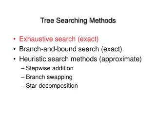
Tree Searching Methods. Exhaustive search (exact) Branch-and-bound search (exact) Heuristic search methods (approximate) Stepwise addition Branch swapping Star decomposition. Exhaustive Search. 12. 12. 13. 13. 13. 12. 13. 13. 12. 13. 11. 13. 13. 13. 13. Searching for trees.

E N D
Tree Searching Methods • Exhaustive search (exact) • Branch-and-bound search (exact) • Heuristic search methods (approximate) • Stepwise addition • Branch swapping • Star decomposition
Exhaustive Search 12 12 13 13 13 12 13 13 12 13 11 13 13 13 13
Searching for trees 1.Generate all 3 trees for first 4 taxa: • Generation of all possible trees
Searching for trees 2. Generate all 15 trees for first 5 taxa: (likewise for each of the other two 4-taxon trees)
Searching for trees 3. Full search tree:
Searching for trees The search tree is the same as for exhaustive search, with tree lengths for a hypothetical data set shown in boldface type. If a tree lying at a node of this search tree has a length that exceeds the current lower bound on the optimal tree length, this path of the search tree is terminated (indicated by a cross-bar), and the algorithm backtracks and takes the next available path. When a tip of the search tree is reached (i.e., when we arrive at a tree containing the full set of taxa), the tree is either optimal (and hence retained) or suboptimal (and rejected). When all paths leading from the initial 3-taxon tree have been explored, the algorithm terminates, and all most-parsimonious trees will have been identified. Asterisks indicate points at which the current lower bound is reduced. Circled numbers represent the order in which phylogenetic trees are visited in the search tree. Branch and bound algorithm:
1 2 2 1 1 3 4 3 3 4 4 2 Stepwise Addition (in a nutshell) 2 1 3
Searching for trees Stepwise addition A greedy stepwise-addition search applied to the example used for branch-and-bound. The best 4-taxon tree is determined by evaluating the lengths of the three trees obtained by joining taxon D to tree 1 containing only the first three taxa. Taxa E and F are then connected to the five and seven possible locations, respectively, on trees 4 and 9, with only the shortest trees found during each step being used for the next step. In this example, the 233-step tree obtained is not a global optimum. Circled numbers indicate the order in which phylogenetic trees are evaluated in the stepwise-addition search.
Stepwise Addition Variants • As Is • add in order found in matrix • Closest • add unplaced taxa that requires smallest increase • Furthest • add unplaced taxa that requires largest increase • Simple • Farris’s (1970) “simple algorithm” uses a set of pairwise reference distances • Random • random permutation of taxa is used to select the order
B C E A D E D A B C Branch swappingNearest Neighbor Interchange (NNI) B C D A E
B A E B D A C F C G D D C E E A F F B G G Branch swappingSubtree Pruning and Regrafting (SPR) a
E D B A F G B A A C C E D B C D D F G E E E D C F A F F G B G G B A C Branch swappingTree Bisection and Reconnection (TBR)
Reconnection limits in TBR Reconnection distances:
Reconnection limits in TBR Reconnection distances: In PAUP*, use “ReconLim” to set maximum reconnection distance
Overview of maximum likelihood as used in phylogenetics • Overall goal: Find a tree topology (and associated parameter estimates) that maximizes the probability of obtaining the observed data, given a model of evolution Likelihood(hypothesis) µProb(data|hypothesis) Likelihood(tree,model) = k Prob(observed sequences|tree,model) [not Prob(tree|data,model)]
C C A G (1) (3) (5) (2) (4) (6) Computing the likelihood of a single tree 1 jN(1) C…GGACA…C…GTTTA…C(2) C…AGACA…C…CTCTA…C(3) C…GGATA…A…GTTAA…C(4) C…GGATA…G…CCTAG…C
C C A G C C A G Prob + Prob A C A A C C A G + … + Prob T T Computing the likelihood of a single tree Likelihood at site j = But use Felsenstein (1981) pruning algorithm
Computing the likelihood of a single tree Note: PAUP* reports -ln L, so lower -ln L implies higher likelihood
Finding the maximum-likelihood tree(in principle) • Evaluate the likelihood of each possible tree for a given collection of taxa. • Choose the tree topology which maximizes the likelihood over all possible trees.
Probability calculations require… • An explicit model of substitution that specifies change probabilities for a given branch length“Instantaneous rate matrix” Jukes-Cantor Kimura 2-parameter Hasegawa-Kishino-Yano (HKY) Felsenstein 1981, 1984 General time-reversible • An estimate of optimal branch lengths in units of expected amount of change ( = rate x time)
Jukes-Cantor (1969) Kimura (1980) “2-parameter” Hasegawa-Kishino-Yano (1985) General-Time Reversible For example:
C C A A A A A A A A C A C C A A A A A A A A C A The Relevance of Branch Lengths
A C B D When does maximum likelihood work better than parsimony? • When you’re in the “Felsenstein Zone” (Felsenstein, 1978)
A B 0.8 0.8 0.1 0.1 0.1 C D A C G T A - 5 6 2 C 5 - 3 8 Substitution rates: G 6 3 - 1 T 2 8 1 - Base frequencies: A=0.1 C=0.2 G=0.3 T=0.4 In the Felsenstein Zone
In the Felsenstein Zone 1 0.8 parsimony 0.6 Proportion correct ML-GTR 0.4 0.2 0 0 5000 10000 Sequence Length
The long-branch attraction (LBA) problem Pattern type 14 A I = Uninformative (constant) A The true phylogeny of 1, 2, 3 and 4 (zero changes required on any tree) A A 23
The long-branch attraction (LBA) problem Pattern type 14 A I = Uninformative (constant) A A II = Uninformative G The true phylogeny of 1, 2, 3 and 4 (one change required on any tree) A A 23
The long-branch attraction (LBA) problem Pattern type 14 A I = Uninformative (constant) A A II = Uninformative G C III = Uninformative G The true phylogeny of 1, 2, 3 and 4 (two changes required on any tree) A A 23
The long-branch attraction (LBA) problem Pattern type 14 A I = Uninformative (constant) A A II = Uninformative G C III = Uninformative G G IV = Misinformative G The true phylogeny of 1, 2, 3 and 4 (two changes required on true tree) A A 23
The long-branch attraction (LBA) problem … but this tree needs only one step G 1 A 2 A 3 G 4
Concerns about statistical properties and suitability of models (assumptions) Consistency If an estimator converges to the true value of a parameter as the amount of data increases toward infinity, the estimator is consistent.
1 3 2 4 When do both methods fail? • When there is insufficient phylogenetic signal...
When does parsimony work “better” than maximum likelihood? • When you’re in the Inverse-Felsenstein (“Farris”) zone A C (Siddall, 1998) D B
Siddall (1998) parameter space a b b a b 0.75 p a Both methods do poorly Parsimony has higher accuracy than likelihood 0 0.75 p b Both methods do well
Parsimony vs. likelihood in the Inverse-Felsenstein Zone 1 B B B B B B B B B B B 0.9 J 15% B 67.5% 0.8 J 0.7 67.5% 0.6 J (expected differences/site) J Accuracy 0.5 J J J J 0.4 J J J J 0.3 0.2 B Parsimony J ML/JC 0.1 0 20 100 1,000 10,000 100,000 Sequence length
Why does parsimony do so well in theInverse-Felsenstein zone? C A C A True synapomorphy A C C C A A A C A Apparent synapomorphies actually due to misinterpreted homoplasy C C C A A A A G G C C
Parsimony vs. likelihood in the Felsenstein Zone 1 J J J J J 0.9 J 0.8 J 0.7 67.5% 67.5% J 0.6 15% Accuracy 0.5 J (expected differences/site) J 0.4 J 0.3 J 0.2 B Parsimony B J ML/JC 0.1 B B 0 B B B B B B B B B 20 100 1,000 10,000 100,000 Sequence length
From the Farris Zone to the Felsenstein Zone A A A C C C D D D B B B A A C C D D B B External branches = 0.5 or 0.05 substitutions/site, Jukes-Cantor model of nucleotide substitution
G H H H H H G 1.0 H G G G G J J J J J J 0.8 0.6 Accuracy 0.4 100 sites J 1,000 sites G J J 10,000 sites H 0.2 J J J J G G H H G H G H G G H 0 H 0.05 0.04 0.03 0.02 0.01 0 0.01 0.02 0.03 0.04 0.05 Farris zon e Length of internal branch ( d ) Felsenstein zone H H 1.0 H H H H G G H H G H G G G 0.8 H J G G J J G 0.6 J J J Accuracy J G J J 0.4 J H G J G J H 100 sites J 0.2 1,000 sites G 10,000 sites H ML/JC 0 0.05 0.04 0.03 0.02 0.01 0 0.01 0.02 0.03 0.04 0.05 Farris zon e Length of internal branch ( d ) Felsenstein zone Simulation results: Parsimony Likelihood
Maximum likelihood models are oversimplifications of reality. If I assume the wrong model, won’t my results be meaningless? • Not necessarily (maximum likelihood is pretty robust)
A B 0.8 0.8 0.1 0.1 0.1 C D A C G T A - 5 6 2 C 5 - 3 8 Substitution rates: G 6 3 - 1 T 2 8 1 - Base frequencies: A=0.1 C=0.2 G=0.3 T=0.4 Model used for simulation...
Among site rate heterogeneity equal rates? Lemur AAGCTTCATAG TTGCATCATCCA …TTACATCATCCA Homo AAGCTTCACCG TTGCATCATCCA …TTACATCCTCAT Pan AAGCTTCACCG TTACGCCATCCA …TTACATCCTCAT Goril AAGCTTCACCG TTACGCCATCCA …CCCACGGACTTA Pongo AAGCTTCACCG TTACGCCATCCT …GCAACCACCCTC Hylo AAGCTTTACAG TTACATTATCCG …TGCAACCGTCCT Maca AAGCTTTTCCG TTACATTATCCG …CGCAACCATCCT • Proportion of invariable sites • Some sites don’t change do to strong functional or structural constraint (Hasegawa et al., 1985) • Site-specific rates • Different relative rates assumed for pre-assigned subsets of sites • Gamma-distributed rates • Rate variation assumed to follow a gamma distribution with shape parameter
. . . . . Performance of ML when its model is violated (another example) Modeling among-site rate variation with a gamma distribution... 0.08 a=200 0.06 a=0.5 a=2 Frequency 0.04 a=50 0.02 0 0 1 2 Rate …can also estimate a proportion of “invariable” sites (pinv)
Performance of ML when its model is violated (another example)