Neural Networks
140 likes | 171 Views
This informative text delves into the intricate world of neural networks and multi-stage regression/classification models. It explores topics such as hidden layer bias units, synaptic weights, activation functions, and the concept of ridge functions in PPR. The text highlights the importance of various activation functions, including the Gaussian radial basis and sigmoid functions. Additionally, it touches on the significance of output functions in regression and classification tasks, shedding light on the rationale behind making the output layer sum-to-one using functions like softmax. The discussion continues with insights on fitting neural networks as function approximators, gradient descent techniques, back-propagation methods, and strategies to prevent overfitting, such as regularization and early stopping. The text also addresses questions related to model training, convergence, model complexity measurement, and the universal approximation capabilities of neural networks, as well as providing historical context and comparisons between neural networks and PPR models.

Neural Networks
E N D
Presentation Transcript
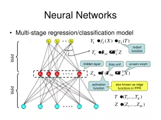
Neural Networks • Multi-stage regression/classification model output function PPR hidden layer bias unit synaptic weight activation function also known as ridge functions in PPR PPR
Activation Function • Gaussian radial basis → radial basis function network • Sigmoid: • differentiable • almost linear around 0 large s small s
Output Function • Regression: • Classification: • Weihao: Any other justification to make output layer sum-to-one using, say, softmax function in Eq. 11.6? • Answer: Think of NN as a function approximator.
Fitting NN (cont’d) • Gradient descent (for regression)
Back-propagation(aka “delta rule”) • Forward pass given/computed values
Back-propagation (cont’d) • Backward pass given/computed values
Back-propagation (cont’d) • Error surface and learning rate • γopt(Θ): optimal learning rate at weights Θ • Assuming quadratic error surface • will NOT converge
Back-propagation (cont’d) • Batch learning vs. online learning • Often too slow • Newton method not attractive (2nd derivative too costly) • Use conjugate gradients, variable metric methods, etc. (Ch. 10, Numerical Recipes in C: http://www.library.cornell.edu/nr/bookcpdf.html)
Back-propagation (cont’d) regularization! • Prevent over-fitting • Start from zero weights • Introducing non-linearity when necessary • Early stopping • Smaller/adaptive learning rates • Convergence guaranteed if
0 0 0 Back-propagation (cont’d) • Joy: … since all parameters for starting are close to 0, how could different starting points ended in models differ that much? • Answer: non-linearity. • Joy: To prevent fitting: is there any way to train the model to the global minimum point and then "prune" it? • Answer: Global minimum is elusive. But the people have tried the idea of ‘pruning’, in weight decay (later) and optimal brain damage:Y. LeCun, J. S. Denker, and S. A. Solla. Optimal brain damage. In D. S. Touretzky, editor, Advances in Neural Information Processing Systems II, pages 598--605. Morgan Kaufmann, San Mateo, CA, 1990.Less ‘salient’ connections can be removed (pruned); saliency ≠ magnitude!
Historical Background • McCulloch & Pitts, 1941: behavior of simple neural networks. • A. Turing, 1948: “B-type unorganized machine” consisting of networks of NAND gates. • Rosenblatt, 1958: two-layer perceptrons. • Minsky & Papert, 1969 (Perceptrons): showing XOR problems for perceptrons; connectionism winter came. • Rumelhart, Hinton & Williams, 1986: first well-known introduction of back-propagation algorithm; connectionism revived.
Model Complexity of NN • Fan: How can we measure the complexity of a NN? … If one NN has many layers but few nodes, another has many nodes but few layers, which one is more complex? …Kevyn: … how can we derive the effective # of degrees of freedom based on the number of iterations we have performed? … • Answer: remember in Ch. 5 we haveand we define - can we do the same for NN?For regression, andbut we have non-linearity inside B!Maybe use Taylor expansion of sigmoid and proceed? (so we’re basically approximating NN using linear models)
NN: Universal Approximator? • Kolmogorov proved any continuous function g(x) defined on the unit hypercube In can be represented asfor properly chosen and .(A. N. Kolmogorov. On the representation of continuous functions of several variables by superposition of continuous functions of one variable and addition.Doklady Akademiia Nauk SSSR, 114(5):953-956, 1957)
NN vs. PPR • NN: parametric version of PPR • less complex σ implies more terms (20-100 vs. 5-10)


