Download
1 / 81
810 likes | 850 Views
Exploring the theory of production, profit maximization, and business organization types for effective decision-making. Learn the key concepts to optimize economic outcomes.

E N D
The Firm and Its Economic Problem • A firm is an institution that hires factors of production and organizes them to produce and sell goods and services. • The Firm’s Goal • A firm’s goal is to maximize profit. • If the firm fails to maximize its profit, the firm is either eliminated or bought out by other firms seeking to maximize profit.
The Firm and Its Economic Problem • Accounting Profit • Accountants measure a firm’s profit to ensure that the firm pays the correct amount of tax and to show it investors how their funds are being used. • Profit equals total revenue minus total cost. • Accountants use Internal Revenue Service rules based on standards established by the Financial Accounting Standards Board to calculate a firm’s depreciation cost.
The Firm and Its Economic Problem • Economic Profit • Economists measure a firm’s profit to enable them to predict the firm’s decisions, and the goal of these decisions in to maximize economic profit. • Economic profit is equal to total revenue minus total cost, with total cost measured as the opportunity cost of production.
The Firm and Its Economic Problem • A Firm’s Opportunity Cost of Production • A firm’s opportunity cost of production is the value of the best alternative use of the resources that a firm uses in production. • A firm’s opportunity cost of production is the sum of the cost of using resources • Bought in the market • Owned by the firm • Supplied by the firm's owner
Information and Organization • Types of Business Organization • There are three types of business organization: • Proprietorship • Partnership • Corporation
Information and Organization • Proprietorship • A proprietorship is a firm with a single owner who has unlimited liability, or legal responsibility for all debts incurred by the firm—up to an amount equal to the entire wealth of the owner. • The proprietor also makes management decisions and receives the firm’s profit. • Profits are taxed the same as the owner’s other income.
Information and Organization • Partnership • A partnership is a firm with two or more owners who have unlimited liability. • Partners must agree on a management structure and how to divide up the profits. • Profits from partnerships are taxed as the personal income of the owners.
Information and Organization • Corporation • A corporation is owned by one or more stockholders with limited liability, which means the owners who have legal liability only for the initial value of their investment. • The personal wealth of the stockholders is not at risk if the firm goes bankrupt. • The profit of corporations is taxed twice—once as a corporate tax on firm profits, and then again as income taxes paid by stockholders receiving their after-tax profits distributed as dividends.
Markets and Firms • Why Firms? • Firms coordinate production when they can do so more efficiently than a market. • Four key reasons might make firms more efficient. Firms can achieve • Lower transactions costs • Economies of scale • Economies of scope • Economies of team production
Markets and Firms • Transactions costs are the costs arising from finding someone with whom to do business, reaching agreement on the price and other aspects of the exchange, and ensuring that the terms of the agreement are fulfilled. • Economies of scale occur when the cost of producing a unit of a good falls as its output rate increases. • Economies of scope arise when a firm can use specialized inputs to produce a range of different goods at a lower cost than otherwise. • Economies of team production • Firms can engage in team production, in which the individuals specialize in mutually supporting tasks.
Production • The theory of the firm describes how a firm makes cost-minimizing production decisions and how the firm’s resulting cost varies with its output. • Production is a process in which firm transform its inputs (factor of production) to output
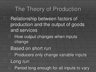
Production function • Q = F( K, L ) • Function showing the highest output that a firm can produce for every specified combination of inputs. • Q= Total Product • K= Capital (Fixed factor of Production) • L=Labor (Variable factor of Production)
The Short Run versus the Long Run • short run Period of time in which quantities of one or more production factors cannot be changed. • long run Amount of time needed to make all production inputs variable. • fixed input Production factor that cannot be varied
PRODUCTION WITH ONE VARIABLE INPUT (LABOR) Average and Marginal Products ●average product Output per unit of a particular input. ●marginal product Additional output produced as an input is increased by one unit. Average product of labor = Output/labor input = q/L Marginal product of labor = Change in output/change in labor input = Δq/ΔL
TPL MPL = TP L APL = MPLAPL EL = Production FunctionWith One Variable Input Total Product TP = Q = f(L) Marginal Product Average Product Production orOutput Elasticity
PRODUCTION WITH ONE VARIABLE INPUT (LABOR) MarginalProduct (∆q/∆L) Amountof Labor (L) Amountof Capital (K) TotalOutput (q) AverageProduct (q/L)
PRODUCTION WITH ONE VARIABLE INPUT (LABOR) The Slopes of the Product Curve Production with One Variable Input The total product curve in (a) shows the output produced for different amounts of labor input. The average and marginal products in (b) can be obtained (using the data in Table 6.1) from the total product curve. At point A in (a), the marginal product is 20 because the tangent to the total product curve has a slope of 20. At point B in (a) the average product of labor is 20, which is the slope of the line from the origin to B. The average product of labor at point C in (a) is given by the slope of the line 0C.
The Law of Diminishing Returns • As additional units of a variable input are combined with a fixed input, after a point the additional output (marginal product) starts to diminish. This is the principle that after a point, the marginal product of a variable input declines.
Increasing Returns MP Diminishing Returns Begins X MP The law of diminishing return
The law of variable proportions states that as the quantity of one factor is increased, keeping the other factors fixed, the marginal product of that factor will eventually decline. This means that upto the use of a certain amount of variable factor, marginal product of the factor may increase and after a certain stage it starts diminishing. When the variable factor becomes relatively abundant, the marginal product may become negative. Assumptions of Law. →Constant technology--- This law assumes that technology does not change throughout the operation of the law. →Fixed amount of some factors.—One factor of production has to be fixed for this law. → Possibility of varying factor proportions—This law assumes that variable factors can be --changed in the short run.
If MP > AP then AP is rising. If MP < AP then AP is falling. MP=AP when AP is maximized.
The three stages of production • Stage I: The range of increasing average product of the variable input. From zero units of the variable input to where AP is maximized • Stage II: The range from the point of maximum AP of the variable to the point at which the MP of is zero. From the maximum AP to where MP=0 • Stage III: The range of negative marginal product of the variable input. From where MP=0 and MP is negative.
In the short run, rational firms should only be operating in Stage II. • Why not Stage III? Firm uses more variable inputs to produce less output • Why not Stage I? Underutilizing fixed capacity Can increase output per unit by increasing the amount of the variable input
What level of input usage within Stage II is best for the firm? The answer depends upon how many units of output the firm can sell, the price of the product, and the monetary costs of employing the variable input.
Production With Two Variable Inputs Isoquants show combinations of two inputs that can produce the same level of output. Firms will only use combinations of two inputs that are in the economic region of production, which is defined by the portion of each isoquant that is negatively sloped.
PRODUCTION WITH TWO VARIABLE INPUTS Isoquants LABOR INPUT ●isoquant Curve showing all possible combinations of inputs that yield the same output.
PRODUCTION WITH TWO VARIABLE INPUTS Isoquants ●isoquant map Graph combining a number of isoquants, used to describe a production function. Figure 6.4 Production with Two Variable Inputs(continued) A set of isoquants, or isoquant map, describes the firm’s production function. Output increases as we move from isoquant q1 (at which 55 units per year are produced at points such as A and D), to isoquant q2 (75 units per year at points such as B) and to isoquant q3 (90 units per year at points such as C and E).
Marginal Rate of Technical Substitution Marginal Rate of Technical Substitution: The absolute value of the slope of the iso-quant. It equals the ratio the marginal products of the two inputs. Slope of iso-quant indicates the quantity of one input that can be traded for another input, while keeping output constant.
Properties of Isoquants Isoquants are negatively sloped A higher Isoquants represent a larger output No two isoquants intersect or touch each other Isoquants are convex to the origin
PRODUCTION WITH TWO VARIABLE INPUTS Diminishing Marginal Returns Production with Two Variable Inputs(continued) Diminishing Marginal Returns Holding the amount of capital fixed at a particular level—say 3, we can see that each additional unit of labor generates less and less additional output.
PRODUCTION WITH TWO VARIABLE INPUTS Substitution Among Inputs ●marginal rate of technical substitution (MRTS) Amount by which the quantity of one input can be reduced when one extra unit of another input is used, so that output remains constant. MRTS = − Change in capital input/change in labor input = − ΔK/ΔL (for a fixed level of q) Marginal rate of technical substitution Like indifference curves, isoquants are downward sloping and convex. The slope of the isoquant at any point measures the marginal rate of technical substitution—the ability of the firm to replace capital with labor while maintaining the same level of output. On isoquant q2, the MRTS falls from 2 to 1 to 2/3 to 1/3.
PRODUCTION WITH TWO VARIABLE INPUTS Production Functions—Two Special Cases Isoquants When Inputs Are Perfect Substitutes When the isoquants are straight lines, the MRTS is constant. Thus the rate at which capital and labor can be substituted for each other is the same no matter what level of inputs is being used. Points A, B, and C represent three different capital-labor combinations that generate the same output q3.
PRODUCTION WITH TWO VARIABLE INPUTS Production Functions—Two Special Cases ●fixed-proportions production function Production function with L-shaped isoquants, so that only one combination of labor and capital can be used to produce each level of output. Fixed-Proportions Production Function When the isoquants are L-shaped, only one combination of labor and capital can be used to produce a given output (as at point A on isoquant q1, point B on isoquant q2, and point C on isoquant q3). Adding more labor alone does not increase output, nor does adding more capital alone. The fixed-proportions production function describes situations in which methods of production are limited.
Optimal Combination of Inputs Isocost lines represent all combinations of two inputs that a firm can purchase with the same total cost.
Isocost Lines • An isocost line is a line that identifies all the combinations of capital and labor, two factor inputs, that can be purchased at a given total cost. • The line intersects each axis at the quantity of that input that the firm could purchase if only that input were purchased. • The slope of an isocost line is (minus) the ratio of input prices, w/r, indicating the relative prices of inputs.
Least Costly Input Combination • A point of tangency between an isocost line and an isoquant show the least costly way of producing a given output level. • Alternatively, a point of tangency shows the maximum output attainable at a given cost as well as the minimum cost necessary to produce that output.
Interpreting the Tangency Points • Golden rule of cost minimization: a rule that says that to minimize cost, the firm should employ inputs in such a way that the marginal product per dollar spent is equal across all inputs MPL/w = MPK/r
If the firm is not producing at a tangency point… • Whenever MPL/w > MPK/r, a firm can increase output without increasing production cost by shifting outlays from capital to labor. • Whenever MPL/w < MPK/r, a firm can increase output without increasing production cost by shifting outlays from labor to capital.
The Expansion Path • The expansion path is a curve formed by connecting the points of tangency between isocost lines and the highest respective attainable isoquants.
Isocost Lines and the Expansion Path [Figure 8.4]
Optimal Combination of Inputs Isocost Lines AB C = $100, w = r = $10 A’B’ C = $140, w = r = $10 A’’B’’ C = $80, w = r = $10 AB* C = $100, w = $5, r = $10
Optimal Combination of Inputs MRTS = w/r
RETURNS TO SCALE ●returns to scale Rate at which output increases as inputs are increased proportionately. ●increasing returns to scale Situation in which output more than doubles when all inputs are doubled. ●constant returns to scale Situation in which output doubles when all inputs are doubled. ●decreasing returns to scale Situation in which output less than doubles when all inputs are doubled.
Optimal Combination of Inputs Effect of a Change in Input Prices
Returns to Scale Constant Returns to Scale Increasing Returns to Scale Decreasing Returns to Scale
RETURNS TO SCALE Describing Returns to Scale Returns to Scale When a firm’s production process exhibits constant returns to scale as shown by a movement along line 0A in part (a), the isoquants are equally spaced as output increases proportionally. However, when there are increasing returns to scale as shown in (b), the isoquants move closer together as inputs are increased along the line.
Empirical Production Functions Cobb-Douglas Production Function Q = AKaLb Estimated using Natural Logarithms ln Q = ln A + a ln K + b ln L