The Theory of Production

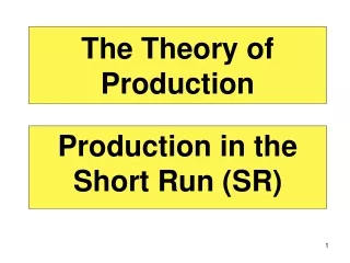
1. The Theory of Production Production in the Short Run (SR)

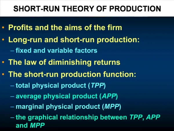
2. Connector • Covered in Economics AS is the make up of a firm’s costs, total costs, fixed costs and variable costs. • These are the costs to the individual firm that it incurs as a result of production. • Write down the definition of the above terms

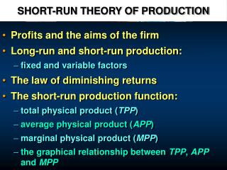
3. Lesson Objectives • Revise definitions and knowledge of costs from AS • Learn the differences between fixed, variable and marginal costs • Understand the shape of the average and marginal cost curves • Understand the theory that explains the short run • Appreciate that different sized firms have different levels of productive efficiency

4. The Big Picture • In this lesson we will start our advanced study of microeconomics by building on your knowledge from AS. • We will look at the costs of production faced by the individual firm and we will analyse them in more depth than you experienced at AS. • We will look at marginal and average costs and revenues and use numerical examples to explain firms’ behaviour. • You will become aware of the diagrammatic presentation of costs curves which we use at A2 and the effect of time on the firms’ costs in terms of short-run.

5. Big Picture • To arrive at the learning outcomes you will do the following: • Listen to teacher demonstrations on PPP • Draw graphs • watch VIDEO • ‘Stretch and challenge’ Questions • Group work • Independent work • Class discussion • Short presentation • Debate economic issues • Demonstration on the board • Pair marking • Advise on examiner’s tip

6. Lesson Outcome • Understand the difference between the short and long run and the theories that underpin them • Be able to use short-run (SR) and long-run (LR) concepts to answer questions • Be able to explain the relationship between average and marginal costs both in words and graphically

7. Total costs Fixed costs Variable costs Short run Long run Marginal Product Average product Increasing marginal returns Diminishing marginal returns Law of diminishing marginal returns Optimum output Productive efficiency Depreciation Semi-variable costs Average fixed cost Average variable cost Average total cost Marginal cost Key Terms

8. Production in the Short Run (SR)

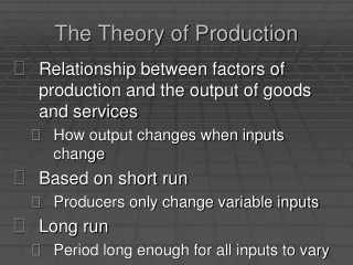
9. Production in the Short Run (SR) • Assume a fictional firm that has been set up to produce reproduction furniture and has hired a factory unit and machinery in order to carry out production. • Initially the firm has incurred some fixed costs in terms of the factory unit and the machinery • The owners of these will expect to be paid for their use from the outset, even though production has not yet started. • Economists study costs over different time periods. These are the short run and the long run.

10. Production in the Short Run (SR) • As the firm commences production of furniture we assume that it is in a short-run situation • where at least one factor remains fixed, • for example, the size of the premises. • To increase its output it will take on extra workers and as it does so it will find, up to a point, • that each worker will add more to the total output than the previous workers.

11. Production in the Short Run • In table 1.1, the marginal product of worker no. 3 is 9 units, • whereas the marginal product of worker no. 4 is 12 units. • This is referred to as increasing marginal returns – where increasing the amount of the variable factor increases output more than proportionately. This has nothing to do with the quality of the workers as we are assuming they are all equally capable

12. Production in the Short Run • As the firm grows and orders increase it will continue to employ more workers and purchase more raw materials. • However, there will come a point • where the premises cannot accommodate extra workers • and their presence will reduce the output of the existing workers.

13. Production in the Short Run • From Table 1.1, marginal product rises up to five workers • each successive worker adds more output than the previous worker. • But with worker number 6MP begins to fall. • However, average productrises and as the MP is above the AP it pulls the average up. • Employment of the 7th worker only adds 3 units of output • as the fixed factors (the size of the factory unit and the number of machine) are now overloaded • as there are too many variable factors for the size of the fixed factor.

14. Production in the Short Run

15. Production in the Short Run • In the short run the firm can only change its rate of output by combining more or less of the variable factors with the fixed factor and the table indicates that: • Initially there are increasing marginal returns to the variable factor so that output rises more than proportionately to the increase in the variable input • Subsequently the firm experiences diminishing marginal returns to the variable input as the increase in output is less than proportional to the increase in labour input. • This sequence of events occurs because the plant is of a fixed size and must eventually become overloaded. • This is referred to as the law of diminishing returns. • This is the ‘law’ that economists use to explain the short run

16. http://www.youtube.com/watch?v=M7rA4VfvdAw&feature=related

17. http://www.youtube.com/watch?v=XqE5inlQCRU

18. Production in the Short RunTable 1.1 indicates the amount produced, the pattern of costs can be inferred from it. • Figure 1.1 illustrates both diminishing and increasing short-run costs where the average total cost curve(ATC) is at its lowest point with the employment of 6 workers. • This is known as the optimum output, the point where the firm has achieved the lowest cost combination between fixed and variable factors. • This is also the point of productive efficiency in the short run as the firm is operating at the minimum average cost.

19. Production in the Short RunTable 1.1 indicates the amount produced, the pattern of costs can be inferred from it. • If the firm decides to increase its output and needs to employ extra workers, beyond six workers it will face increasing costs and will no longer be productively efficient.

22. Production in the Short RunTable 1.1 indicates the amount produced, the pattern of costs can be inferred from it. • Figure 1.2 indicates the revenues of the firm (output X price) and average revenue will be at maximum at an output of 60 units where six worker are employed. • If the firm produces more output its average revenue start to fall. • In the short run we have encountered a number of costs: fixed, variable and marginal.

23. Production in the Short Run

24. How do marginal returns affect marginal costs?Diagrammatically, the link between marginal returns (or marginal product) and marginal costs isshown in Figure 3.2 below. • This question provides the opportunity to distinguish between a production function and a cost • function, and also between marginal product and marginal costs. In the answer to Question 2, a • firm’s short-run production function was: • Q = f(K–, L) • Taking this one stage further, the marginal returns or marginal product (MPL) of labour can be • written as: • MPL = ΔQ/ΔL • In a similar way, the firm’s short-run cost function is: • C = f(Q) • and marginal costs of production (MC) are: • MC = ΔC/ΔQ • Diagrammatically, the link between marginal returns (or marginal product) and marginal costs is shown in Figure 3.2 below. • To start with, as it employs labour, the firm benefits from the increasing marginal productivity of labour. This is shown by the rising section of the MP curve in the upper panel of Figure 3.2. Extra workers add more to total output than previous workers employed, but the wage cost of employing an extra worker remains the same. As a result, the total cost of producing output rises at a slower rate than output itself, and this causes the marginal cost (MC) of producing an extra unit of output to fall. The increasing marginal productivity of labour (shown by the positive slope of the marginal product curve in the upper panel of Figure 3.2) thus causes marginal cost (in the lower panel) to fall. • However, once the law of diminishing marginal productivity sets in, marginal cost rises with output. The wage cost of employing an extra worker is still the same, but each extra worker is now less productive than the previous worker who joined the labour force. The total cost of production rises faster than output, so the marginal cost of producing output also rises.

27. Fixed Costs • In the short run, because at least one factor of production is fixed, output can be increased only by adding more variable factors • Hence we make a distinction between fixed and variable costs

28. Understanding Short Run Costs Short run costs Fixed Costs Variable Costs AC, MC and AVC

29. Fixed factor inputs

30. Production in the Short Run Fixed costs • Fixed costs will not vary with output in the short run and they are sometimes called overhead or indirect costs. • They are looked upon as contractual, that is, enforceable in a court of law, and usually consist of payments of on building and machinery. • Fixed costs have to be paid whether the firm produces nothing or runs the plant 24 hours per day, and as a result, in a cost table fixed costs will be shown even when the firm is not producing any output, for example, £180 at zero output in Table 1.2. • In addition to those mentioned, typical example of fixed costs are rents, salaries of permanent employees and depreciation.

31. Examples of fixed costs for this business? (Speedferries)

32. Fixed Costs • Fixed costs • These do not vary directly with the level of output i.e. they are treated as independent of production • Examples of fixed costs include the rental costs of buildings, the costs of leasing or purchasing capital equipment such as plant and machinery, the costs of full-time contracted salaried staff, the costs of meeting interest payments on loans, the depreciation of fixed capital (due solely to age) and also the costs of business insurance

33. 15

34. Fixed Cost Curves Costs Total Fixed Cost Output Fixed costs (FC) are totally independent of output and must be paid out even if the production stops. Capital intensive industries with a high ratio of fixed to variable costs offer scope for economies of scale AFC = Fixed Costs (FC) / Output (Q).

35. Fixed Cost Curves AFC = Fixed Costs (FC) / Output (Q). Costs Total Fixed Cost Average Fixed Cost Output Average fixed costs must fall continuously as output increases because fixed costs are being spread over a higher level of production. In industries where the ratio of fixed to variable costs is extremely high, there is great scope for a business to exploit lower fixed costs per unit if it can produce at a big enough size

36. Production in the Short Run Variable costs • In contrast with fixed costs, variable costs vary directly with output. • Increasing output will require an increase in such things as raw materials, power and labour. • The variable costs of a firm are zero when there is no output, and increase and decrease as output rises and falls. • When the firm is closed due to, • for example, in a holiday period, variable costs will be zero as production is not taking place. • Variable costs are sometimes called unit-level costs as they vary with the number of units produced. • When the firm is closed due to, • for example, in a holiday period, variable costs will be zero as production is not taking place.

37. Variable Costs • Variable costs are business costs that vary directly with output • Examples of variable costs include the costs of intermediate raw materials and other components, the wages of part-time staff or employees paid by the hour, the costs of electricity and gas and the depreciation of capital inputs due to wear and tear. • Total variable cost rises as output increases • Average variable cost (AVC) = total variable costs (TVC) /output (Q)

38. Production in the Short Run Semi-variable costs • These are costs which have both a fixed cost and variable cost element. • An electricity bill may include elements that are fixed (such as the fixed or standing, charge for supplying the service) • And elements that are variable (such as the amount of electricity used by machinery during the production process).

40. Production in the Short Run • Figure 1.3 shows the total cost curves for a particular firm. • Fixed costs remains at £180 over the range of output produced while costs increase as output increases. • The addition of fixed and variablecostsgives the total cost.

41. Production in the Short Run 15 • The first three columns of the table indicate the total costs • the second three columns are average costs • the last column shows the marginal cost, which is the cost of producingthe extra unit of output.

42. Production in the Short Run 15 • Total costs comprise total fixed costs and total variable costs. • Average fixed cost(AFC) can be found by dividing the total fixed costs by the number produced, and diminishes quite rapidly as the cost is spread over an increasing number of units. • Thus the AFC of unit 2 is TFC(180)÷ 2 = 90 whereas by the time output has increased to nine units AFC has fallen to 20.

43. Production in the Short Run 15 • In contrast, average variable cost(AVC), • TVC divided by the number product • AVC increases as output increases (as variable costs increase with output). • Thus the AVC of unit 1 is 15 but has increased to 190 by unit 9.

44. Production in the Short Run 15 • Average total cost(ATC) is total cost divided by the number produced • ATCdeclines as the fixed cost is spread over more units but then increases as the growth in variable costs is greater than the fall in fixed costs. • For unit 1 ATC is 195, falling to 120 for unit 4 but then rising as output increases and reaches 210 by unit 9.

45. Production in the Short Run 15 Marginal cost (MC) is the amount added to the total cost of production by the next unit of output – the cost of producing one more unit. • The marginal cost is calculated by taking the total cost and deducting the total cost of the previous unit • for example, the total cost of producing six units is £828; the total cost of producing five units is £645. • The MC is therefore the difference between them, £183, and the actual cost of producing the sixth unit. . The marginal cost is calculated by taking the total cost and deducting the total cost of the previous unit

46. Marginal Cost (MC) • Marginal cost is the change in total costs from increasing output by one extra unit. • The marginal cost of an extra unit of output is linked with the marginal productivity of labour • If marginal product is falling, assuming the cost of employing extra units of labour is constant the extra costs of these units of output will rise • There is an inverse relationship between marginal product and marginal cost. The law of diminishing returns implies that the marginal cost of production will rise as output increases. Eventually, rising marginal cost will lead to a rise in average total cost. This happens when the rise in AVC is greater than the fall in AFC as output (Q) increases

47. The Marginal Cost Curve Marginal Cost (MC) Costs Output The law of diminishing returns implies that the marginal cost of production will rise as output increases. Eventually, rising marginal cost will lead to a rise in average total cost

49. An increase in marginal costs MC2 Costs MC1 Output

50. Production in the Short Run This information can be produced in diagrammatic form and figure 1.4 shows three average cost curve: total, variable and fixed, as well as the marginal cost curve. 15