Download
1 / 54
540 likes | 564 Views
Explore the concept of transformations in computer graphics, including affine transformations and linear combinations of vectors. Learn how to scale, rotate, and translate objects in 2D and 3D, and how to use transformations in designing graphics and animations. Discover the graphics pipeline and the role of transformations in creating images.

E N D
Transformations of objects Computer graphics
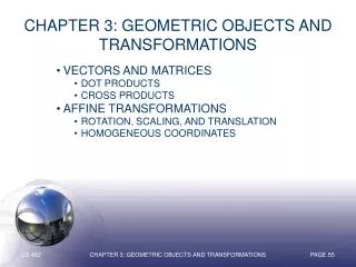
Transformations • We have been using the window to viewport transformation to scale and translate objects in the world window to their size and position in the viewport. • Now, we build on this idea, and gain more flexible control over the size, orientation, and position of objects of interest. • This is achieved through the powerful affine transformation.
Linear Combinations of Vectors • v1 ± v2 = (v1x ± v2x, v1y ± v2y, v1z ± v2z) • sv= (svx, svy, svz) • A linear combination of the m vectors v1, v2, …, vm is w = a1v1 + a2v2 + … + amvm. • Example: 2(3, 4,-1) + 6(-1, 0, 2) forms the vector (0, 8, 10).
Affine and Convex Combinations • The linear combination becomes an affine combination if a1 + a2 + … + am = 1. • Example: 3a + 2 b - 4 c is an affine combination of a, b, and c, but 3 a + b - 4 c is not. • (1-t) a + (t) b is an affine combination of a and b. • The affine combination becomes a convex combination if ai ≥ 0 for 1 ≤ i ≤ m. • Example: .3a+.7b is a convex combination of a and b, but 1.8a -.8b is not.
Example of Affine Transformations • The house has been scaled, rotated and translated, in both 2D and 3D.
Using Transformations • The arch is designed in its own coordinate system. • The scene is drawn by placing a number of instances of the arch at different places and with different sizes.
Using Transformations (2) • In 3D, many cubes make a city.
Using Transformations (3) • The snowflake exhibits symmetries. • We design a single motif and draw the whole shape using appropriate reflections, rotations, and translations of the motif.
Using Transformations (4) • A designer may want to view an object from different vantage points. • Positioning and reorienting a camera can be carried out through the use of 3D affine transformations.
Using Transformations (5) • In a computer animation, objects move. • We make them move by translating and rotating their local coordinate systems as the animation proceeds. • A number of graphics platforms, including OpenGL, provide a graphics pipeline: a sequence of operations which are applied to all points that are sent through it. • A drawing is produced by processing each point.
The OpenGL Graphics Pipeline • This version is simplified.
Graphics Pipeline (2) • An application sends the pipeline a sequence of points P1, P2, ... using commands such as: glBegin(GL_LINES); glVertex3f(...); // send P1 through the pipeline glVertex3f(...); // send P2 through the pipeline ... glEnd(); • These points first encounter a transformation called the current transformation (CT), which alters their values into a different set of points, say Q1, Q2, Q3.
Graphics Pipeline (3) • Just as the original points Pi describe some geometric object, the points Qi describe the transformed version of the same object. • These points are then sent through additional steps, and ultimately are used to draw the final image on the display.
Transformations • Transformations change 2D or 3D points and vectors, or change coordinate systems. • An object transformation alters the coordinates of each point on the object according to the same rule, leaving the underlying coordinate system fixed. • A coordinate transformation defines a new coordinate system in terms of the old one, then represents all of the object’s points in this new system. • Object transformations are easier to understand, so we will do them first.
Transformations (2) • A (2D or 3D) transformation T( ) alters each point, P into a new point, Q, using a specific formula or algorithm: Q= T(P).
Transformations (3) • An arbitrary point P in the plane is mapped to Q. • Q is the image of P under the mapping T. • We transform an object by transforming each of its points, using the same function T() for each point. • The image of line L under T, for instance, consists of the images of all the individual points of L.
Transformations (4) • Most mappings of interest are continuous, so the image of a straight line is still a connected curve of some shape, although it’s not necessarily a straight line. • Affine transformations, however, do preserve lines: the image under T of a straight line is also a straight line.
Transformations (5) • We use an explicit coordinate frame when performing transformations. • A coordinate frame consists of a point O, called the origin, and some mutually perpendicular vectors (called i and j in the 2D case; i, j, and k in the 3D case) that serve as the axes of the coordinate frame. • In 2D,
Transformations (6) • Recall that this means that point P is at location = Pxi + Pyj + O , and similarly for Q. • Px and Py are the coordinates of P. • To get from the origin to point P,move amount Px along axis i and amount Py along axis j.
Transformations (7) • Suppose that transformation T operates on any point P to produce point Q: or Q = T(P). • T may be any transformation: e.g.,
Transformations (8) • To make affine transformations we restrict ourselves to much simpler families of functions, those that are linear in Px and Py. • Affine transformations make it easy to scale, rotate, and reposition figures. • Successive affine transformations can be combined into a single overall affine transformation.
Affine Transformations • Affine transformations have a compact matrix representation. • The matrix associated with an affine transformation operating on 2D vectors or points must be a three-by-three matrix. • This is a direct consequence of representing the vectors and points in homogeneous coordinates.
Affine Transformations (2) • Affine transformations have a simple form. • Because the coordinates of Q are linear combinations of those of P, the transformed point may be written in the form:
Affine Transformations (3) • There are six given constants: m11, m12, etc. • The coordinate Qx consists of portions of both Px and Py, and so does Qy. • This combination between the x- and y-components also gives rise to rotations and shears.
Affine Transformations (4) • Matrix form of the affine transformation in 2D: • For a 2D affine transformation the third row of the matrix is always (0, 0, 1).
Affine Transformations (5) • Some people prefer to use row matrices to represent points and vectors rather than column matrices: e.g., P = (Px, Py, 1) • In this case, the P vector must pre-multiply the matrix, and the transpose of the matrix must be used: Q = P MT.
Affine Transformations (6) • Vectors can be transformed as well as points. • If a 2D vector v has coordinates Vx and Vy then its coordinate frame representation is a column vector with third component 0.
Affine Transformations (7) • When vector V is transformed by the same affine transformation as point P, the result is • Important: to transform a point P into a point Q, post-multiply M by P: Q = M P.
Affine Transformations (8) • Example: find the image Q of point P = (1, 2, 1) using the affine transformation
Geometric Effects of Affine Transformations • Combinations of four elementary transformations: (a) a translation, (b) a scaling, (c) a rotation, and (d) a shear (all shown below).
Translations • The amount P is translated does not depend on P’s position. • It is meaningless to translate vectors. • To translate a point P by a in the x direction and b in the y direction use the matrix: • Only using homogeneous coordinates allow us to include translation as an affine transformation.
Scaling • Scaling is about the origin. If Sx = Sy the scaling is uniform; otherwise it distorts the image. • If Sx or Sy < 0, the image is reflected across the x or y axis. • The matrix form is
Example of Scaling • The scaling (Sx, Sy) = (-1, 2) is applied to a collection of points. Each point is both reflected about the y-axis and scaled by 2 in the y-direction.
Types of Scaling • Pure reflections, for which each of the scale factors is +1 or -1. • A uniform scaling, or a magnification about the origin: Sx = Sy, magnification |S|. • Reflection also occurs if Sx or Sy is negative. • If |S| < 1, the points will be moved closer to the origin, producing a reduced image. • If the scale factors are not the same, the scaling is called a differential scaling.
Rotation • Counterclockwise around origin by angle θ:
Deriving the Rotation Matrix • P is at distance R from the origin, at angle Φ; then P = (Rcos(Φ), Rsin(Φ)). • Q must be at the same distance as P, and at angle θ + Φ: Q =(R cos(θ + Φ), R sin(θ + Φ)). • cos(θ+ Φ) = cos(θ) cos(Φ) - sin(θ) sin(Φ); sin(θ+ Φ) = sin(θ) cos(Φ) + cos(θ) sin(Φ). • Use Px = Rcos(Φ) and Py = Rsin(Φ).
Shear • Shear H about origin: x depends linearly on y in the figure. • Shear along x: h ≠ 0, and Px depends on Py (for example, italic letters). • Shear along y: g ≠ 0, and Py depends on Px.
Inverses of Affine Transformations • det(M) = m11*m22 - m21*m12 0 means that the inverse of a transformation exists. • That is, the transformation can be "undone“. • M M-1 = M-1M = I, the identity matrix (ones down the major diagonal and zeroes elsewhere).
Inverse Translation and Scaling • Inverse of translation T-1: • Inverse of scaling S-1:
Inverse Rotation and Shear • Inverse of rotation R-1 = R(-θ): • Inverse of shear H-1: generally h=0 or g=0.
Composing Affine Transformations • Usually, we want to apply several affine transformations in a particular order to the figures in a scene: for example, • translate by (3, - 4) • then rotate by 30o • then scale by (2, - 1) and so on. • Applying successive affine transformations is called composing affine transformations.
Composing Affine Transformations (2) • T1( ) maps P into Q, and T2( ) maps Q into point W. Is W = T2(Q) = T2(T1(P))affine? • Let T1=M1 and T2=M2, where M1 and M2 are the appropriate matrices. • W = M2(M1P)) = (M2M1)P =MP by associativity. • So M = M2M1, the product of 2 matrices (in reverse order of application), which is affine.
Composing Affine Transformations: Examples • To rotate around an arbitrary point: translate P to the origin, rotate, translate P back to original position. Q = TP R T-P P • Shear around an arbitrary point: Q = TP H T-P P • Scale about an arbitrary point: Q = TPST-P P
Composing Affine Transformations (Examples) • Reflect across an arbitrary line through the origin O: Q = R(θ) S R(-θ) P • The rotation transforms the axis to the x-axis, the reflection is a scaling, and the last rotation transforms back to the original axis. • Window-viewport: Translate by -w.l, -w.b, scale by A, B, translate by v.l, v.b.
Properties of 2D and 3D Affine Transformations • Affine transformations preserve affine combinations of points. • W = a1P1 + a2P2 is an affine combination. • MW = a1MP1 + a2MP2 • Affine transformations preserve lines and planes. • A line through A and B isL(t) = (1-t)A + tB, an affine combination of points. • A plane can also be written as an affine combination of points: P(s, a) = sA + tB +(1 – s – t)C.
Properties of Transformations (2) • Parallelism of lines and planes is preserved. • Line A + bt having direction b transforms to the line given in homogeneous coordinates by M(A + bt) = MA + Mbt, which has direction vector Mb. • Mb does not depend on point A. Thus two different lines A1+ bt and A2 + bt that have the same direction will transform into two lines both having the direction, so they are parallel. • An important consequence of this property is that parallelograms map into other parallelograms.
Properties of Transformations (3) • The direction vectors for a plane also transform into new direction vectors independent of the location of the plane. • As a consequence, parallelepipeds map into other parallelepipeds.
Properties of Transformations (4) • The columns of the matrix reveal the transformed coordinate frame: • Vector i transforms into column m1, vector j into column m2, and the originO into point m3. • The coordinate frame (i, j, O) transforms into the coordinate frame (m1, m2, m3), and these new objects are precisely the columns of the matrix.
Properties of Transformations (5) • The axes of the new coordinate frame are not necessarily perpendicular, nor must they be unit length. • They are still perpendicular if the transformation involves only rotations and uniform scalings. • Any point P = Pxi + Pyj + O transforms into Q = Pxm1 + Pym2 + m3.