SEARCH

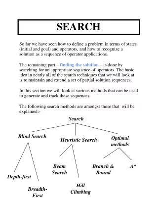
1. SEARCH So far we have seen how to define a problem in terms of states (initial and goal) and operators, and how to recognize a solution as a sequence of operator applications. The remaining part – finding the solution – is done by searching for an appropriate sequence of operators. The basic idea in nearly all of the search techniques that we will look at is to maintain and extend a set of partial solution sequences. In this section we will look at various methods that can be used to generate and track these sequences. The following search methods are amongst those that will be explained:- Search Blind Search Optimal methods Heuristic Search Beam Search Branch & Bound A* Depth-first Hill Climbing Breadth-First

2. The 8-Puzzle The state description specifies the location of each numbered square and the position of the blank. The initial state is usually a random jumble of the numbered squares while the goal state is usually some particular configuration such as is shown above. The operators allow the blank to be moved left, right, up or down. The solution cost is simply the number of moves between the initial and goal states. Goal State Initial State

3. W SR CG SC FA CS S A R E SG L Search Trees In order to explain many techniques we will look at the problem of route planning, in particular planning a route from Clonskeagh Gate to Stillorgan Gate in the following map of UCD. UCD MAP (The State Space) Clonskeagh Gate Dual Carriageway In this problem the states are the locations on the map; the map is the state space. The initial state is GC and the goal state is the SG. There is one operator, Move, that allows one to get from state x to state y so long as there is a edge on the map connecting x and y.

4. A R CG SC S SR W CS L FA SG FA R CS L SG A E E Cont… If we try to find all possible paths from CG then we will certainly find a path to SG, because one does exist. We are in effect transforming the map (which is of course a graph) into a search tree. Each node in this tree represents a path (not a state) even though locations are a more convenient node label – cycles are ignored. Search methods start out with no knowledge about the size of these trees. Accordingly it is crucial to use a search method that is likely to develop the smallest number of paths. It is important to distinguish between the state space and the search tree. These are only 12 nodes in the UCD state space, one for each location. But there can be an infinite number of search tree nodes (if we permit cycles) and even in the non-cycling search tree above, there are 20 nodes, representing 20 non-cycling paths.

5. GRAPH THEORY Structures for State Space Search: A graph is a set of nodes and arcs that connect them. A labeled graph has one or more descriptors (labels) attached to each node that distinguish that node from any other node in the graph. A graph is directed if arcs have an associated directionality. The arcs in a directed graph are usually drawn as arrows or have an arrow attached to indicated directions. A path through a graph connects a sequence of nodes through successive arcs. The path is represented by an ordered list that records the nodes in the order they occur in the path. A rooted graph has a unique node, called the root, such that there is a path from the root to all nodes within the graph. In drawing a graph (rooted), the root is usually drawn at the top of the page, above the other nodes. A tree is a graph in which two nodes have at most one path between them. Trees often have roots, in which case they usually drawn with the root at the top, like a rooted graph. Because each node in a tree has only one path of access from any other node, it is impossible for a path to loop or cycle continuously through a sequence of nodes.

6. TIC TAC TOE The states in the space are all the different configurations of Xs and Os that the game can have. Of course, although there are 39 ways to arrange {blank, X,O} in nine spaces, most of them could never occur in an actual game. Arcs are generated by legal moves of the game, alternating between placing an X and an O in an unsed location. The state space is a graph rather than a tree, as some states on the third and deeper levels can be reached by different paths. However, there are no cycles in the state space, because the directed arcs of the graph do not allow a move to be undone. It is impossible to “go back up”the structure once a state has been reached. No checking for cycles in path generation is necessary. A graph structure with this property is called directed acyclic graph graph and is common in state space search. The state space representation provides a means of determining the complexity of the problem. In tic-tac-toe, there are nine first moves with eight possible responses to each of them, followed by seven and so on… 9! Different paths can be generated. Chess: 10120 possible game paths Checkers: 1040

7. Strategies for State Space Search • Data – driven search or forward chaining The problem solver begins with the given facts of the problem and a set of legal moves or rules for changing state. Search proceeds by applying rules to facts to produce new facts, while are in turn used by the rules to generate more new facts. This process continues until it generates a path that satisfies the goal condition. • Goal driven or backward chaining Alternative approach: take the goal that we want to solve. See what rules or legal moves could be used to generate this goal and determine what conditions must be true to use them. These conditions become the new goals or sub goals for the search. Search continues, working backward through successive sub goals until it works back to the facts of the problem.

8. Implementing Graph Search A problem solver must find a path from a start state to a goal through the space search. Backtracking is a technique for systematically trying all paths through a state space. Backtracking search begins at the start state and pursues a path until it reaches either a goal or a dead end. If it finds a goal, it quits and returns the solution path. If it reaches a dead end, it “backtracks” to the most recent node on the path, having unexamined siblings and continues down one of these branches. A B C D E F G H I J

9. HEURISTIC SEARCH In state space search, heuristics are formalized as rules for chasing those branches in a state space that are most likely to lead to an acceptable problem solution. Ai problem solvers employ heuristics in two basic situations: • A problem may not have an exact solution because of inherent ambiguities in the problem statement or available data • A problem may have an exact solution, but the computational cost of finding it may be prohibitive Evaluation function: f(n) = g(n) + h(n) g(n): measures the actual length of the path from any state n to the start state h(n): a heuristic estimate of the distance from state n to a goal f(n): evaluation function!

10. SC R CS E A R CG SR A W SG FA CS L E FA L S SG Breadth-First Search Breadth-first search traverses a tree in a left-to-right, top-to-bottom fashion. It does this by expanding all of the nodes on a particular level before moving down to the next level. The search is complete. It is also optimal so long as the solution is a non-decreasing function of node depth. Queuing function: Queue new paths at end of queue. Success

11. SC R CS E A R CG SR A W SG FA CS L E FA L S SG Depth-First Search Depth-first search traverses a search tree in a top-to-bottom, left to right fashion. It does this by expanding the left-most open node and working downward fro that node until a leaf node is encountered. If no solution is found on this path then search continues from next lowest, left-most, unexpanded (closed) node. Queuing function: Queue new paths at start of queue. Success

12. Random Queuing Depth-first search is a good idea if you are confident that all partial paths either reach dead ends or become complete solutions at reasonable depths. In contrast breadth-first search can work well when this is not the case, even in trees that are infinitely deep. But breadth first methods are wasteful if all goal nodes are reached at more or less the same depths or if the branching factor is large (in fact even moderate branching factors result in exponential growth). If you have no idea about the topology of the search tree – for example, if you do not know the branching factor or if you cannot rule out the possibility of unmanageably deep solutions paths – then the idea or random queuing offers a pragmatic middle-ground between depth – first and breadth – first methods. In this type of search paths are not added at the start or end of the queue. Instead they are inserted in a random queue position; this is often referred to as non-deterministic search. The effect is that search tree nodes are expanded at random. The search is equally likely to deepen as it is to broaden. Queuing Function: Queue new paths at random positions in queue

13. Depth-Limited Search This search technique avoids the pitfalls of depth-first search by imposing a limit to prevent search from going beyond a certain depth. For example, in the UCD problem we know that no solution will need more than 11 steps because there are only 12 locations. So we can use 11 as a limit and then we need not consider the problem of following infinitely deep paths – we do not have to worry about cycles. We can implement this type of search in a number of ways. One is to modify our operator descriptions to take account of the limit: - Move(x,y) iff Edge(x,y) and Depth < l (depth limit) iWth this new operator set the search method is complete, but it is still not optimal. However it is only complete if we choose an appropriate limit because the search will no longer follow infinitely long paths through the tree, and so will always return to other more promising paths. Of course if the required solution is actually l+1 steps deep then it will never be found. From a complexity viewpoint the method is similar to the standard depth-first procedure, but with the new depth limit playing the role of the maximum tree depth.

14. SC SC CS SC S CG W CG CG CG SR S L l = 0 Iterative - Deepening It is often difficult to find a good search limit to use with depth-limiting methods. For example, choosing 11 for the UCD problem ignores the fact that any location can be reached from any other location in at most 8 steps. This number is the diameter of the state space and provides a much better depth limit. However for most problems the state space diameter is not at all obvious until the problem has been fully solved and the state space fully exposed. Iterative-deepening tries all possible limits from 0 to infinity. Basically the depth-limited search procedure is wrapped in an outer loop that iterates over all possible depth limits, terminating only when a solution is found. l = 2 l = 1 l = 3

15. Search Costs There are two important costs to consider with respect to search-based problem solving: • Search Cost – The cost of finding a solution • Solution Costs – The cost of using this solution Different search techniques offer different guarantees with regards to both of these costs. In general the longer one spends searching, the better resulting solution; that is, high search costs usually mean low solution costs. Depending on the type of problem and the way in which the solution will be used search may or may not be a good idea, and more importantly one particular type of search may be preferred over another. Very briefly, if the solution found is to be applied or used on a regular basis then it is important that this solution be as efficient as possible, even f it means sacrificing search time. In other words solution cost should be minimal at the expense of a high search cost. On the other hand if the problem is a one-off then optimizing the solution cost may no longer be a priority. Instead optimizing the search cost may be the number one concern.

16. Evaluation Concerns Search methods can be usefully compared in terms of the following characteristics: • Time complexity: How long will it take to find a solution? This is related to search cost • Space complexity: How much memory will be used? • Completeness: When success is possible, is it guaranteed? With regards to the complexity characteristics, time and space complexity are measured in terms of the number of nodes that need to be examined (expanded) and held in memory respectively. These values are computed using information such as the branching factor of the tree (commonly referred to as “b”) and the maximum depth of the tree (usually represented by “d”); if a tree has a branching factor of b then every non-leaf (interior) node has b children.

17. BLIND SEARCH Blind search methods have no way of judging which partial path is likely to lead to a solution and which is not so they try to systematically follow all paths in the hope that one will succeed. • Form a one element queue consisting of a zero-length path that contains only the initial state (the root). • Until the first path in the queue terminates at the goal state or the queue is empty. • Remove the first path from the queue • Create new paths by extending the first path to all successor states of its terminal state • Reject all new paths with cycles • Add the new paths to the queue using to the queuing function • If the goal state is found the announce success; otherwise announce failure Blind search methods differ only in the way that they add new paths to the search queue

18. This strategy combines the advantages of depth-first and breadth-first search. It is complete and optimal (in the same sense as breadth-first search) and it benefits from the modest memory requirements of depth-first search. Moreover, the order of state expansion (time complexity) is the same as breadth-first methods except that some states are expanded multiple times. In reality this repetition of work is not as inefficient as it sounds. This may seem counter-intuitive but it can be understood when we recognize that in a search tree exhibiting the properties of exponential growth, the vast majority of the nodes reside at the leaves, that is at level 1. The iterative deepening method builds l+1 search trees each a level deeper than the last. This means that the while the root node is expanded l+1 times the level l leaves are expanded only once – during the last (l+1th) iteration. The number of expansions for a depth-limited search is computed as follows; one expansion for the root, b for the level a nodes, b2 for the level 3 nodes and so on… 1+b+ b2 + … + bl expansions {= 111,111 if b=10, l=5} In iterative deepening the number of expansions is computed as follows . . . (l+1)1 + (1)b + (l-1) b2 + …+ bl expansions {123,456 if b=10, l=5; an increase of only 11%}

19. A note on repeated states Up until now we have all but ignored one of the most important complications to the search process: wasting search effort by exploring states that have already been visited earlier on during the search. For some problems repeated states cannot occur. However in many problems they are unavoidable. For instance, this happens if the search operators are reversible, e.g. during route finding we can move from x to y or from y to x. in such cases, while the state space is finite, the search trees are finite. If we can prune away repeated states however we can greatly reduce the size of the search tree. Note that in our examples up until now we have presented a search tree which is finite, only because its repeated states have been removed. So how can we prevent repeated states from occurring? • Never extend a path to a state that you have just come from. This option is the simplest and only avoids certain types of repetition • Avoid paths with cycles by checking whether a new state has appeared any where in the current path. This avoids cycles within individual paths but ignores the possibility of state repetition across paths • Do not generate any state that has already been visited, irrespective of the path. This option may or may not be desirable, consider the route finding problem…

20. HEURISTIC SEARCH Blind search methods are simple but they are often impractical. They make no attempt to reduce either the search cost of a problem or its solution cost. Heuristic methods on the other hand do at least try to address the search cost issue. The basic idea is that search efficiency may improve drastically if the most promising search paths are explored first. Heuristic functions allow us take advantage of this by providing a means of ordering paths for exploration. For example in the UCD example straight-line distance might be used as the heuristic, favoring paths whose terminal nodes are closer to SG as the crow flies than other paths. The basic heuristic search algorithm is exactly the same as the blind search algorithm with one exception. A heuristic evaluation function is provided so that new paths can be stored before they are added to the search queue.

21. HeuristicSearch(initial, goal, queuing-fn,eval-fn) • Form a one element queue consisting of a zero-length path that contains only the initial state (the root). • Until the first path in the queue terminates at the goal state or the queue is empty. • Remove the first path from the queue • Create new paths by extending the first path to all successor states of its terminal state • Reject all new paths with cycles • Sort the new paths according to the evaluation function • Add the new paths to the queue using to the queuing function • If the goal state is found the announce success; otherwise announce failure Note that these methods sort the paths before they are added to the queue, therefore the entire queue may not be properly sorted at a given instance.

22. SC R CS R CG SR W A SG FA CS L A E E FA L S SG Hill Climbing Evaluation heuristics turn depth-first search into hill climbing. The evaluation function is applied to each new path to measure the “distance”between the path’s terminal state and the goal state. The closer the path is to the goal the better its evaluation result. Below is a trace of hill climbing through the UCD search tree using the straight line distance heuristic:

23. The hill-climbing procedure works by making tentative local changes to its position in the search space and by following those moves that result in the most beneficial state change. This works well when the goal is instantly recognizable, for example, reaching SG. However problems can occur when the goal is nor loosely defined. For example think of a similar television tuning problem. There are two tuning controls, color and contrast and your own subjective heuristic for picture quality. Hill climbing works by making small adjustments to color an contrast and committing to the best one. Eventually a picture quality will be attained that is superior to the quality of neighboring states. You assume that you have found the best picture so your search stops. We can think of this type of search problem in geometrical terms – two parameters to adjust means that we have a 2D search space. In addition different points in this space will have different heights representing their evaluation result. Global maximum Local maximum Quality Contrast Color

24. The Foothill problem:- often there are peaks in the search space that represent local maxima rather than the global maximum. The search process may reach a point where local changes only degrade the quality value and so search may stop under the assumption that an optimal state has been found, when really we have only found a local maxima. One solution to this problem is to introduce of non determinism. The idea is that random steps in random directions may lead the search away from local maxima and nearer to a global maximum. The Plateau problem:- If the search space contains a large flat region (a plateau) then local changes will bring about no change to the quality function and so the search process has no way of knowing how to proceed. Solutions to this problem can include a change of evaluation function so as to transform an apparently level search space into a more strongly featured one. The Ridge problem:- The search space may contain ridges of high quality states which fall off steeply to low quality states on either sides. It may not be possible to accurately follow narrow ridges if the search operators are not fine-grained enough – the result can be an oscillating search.

25. SC R CS R CG SR W A SG FA CS L A E E FA L S SG Beam Search Beam search is like breadth first search in that it proceeds in a level by level fashion. However it avoids the space complexity of breadth-first by limiting the number of nodes it expands at each level. In effect it is a breadth-limiting search where w is used to represent the breadth limit. This essentially reduces the branching factor of the graph from b to w and presumably b> > w. Again a heuristic function is used to judge which are the best w nodes to expand at a particular level:

26. OPTIMAL SEARCH The main issue that heuristic methods are designed to address is that of search cost – they try to improve the time needed to find a solution by using heuristic functions to judge which part of the search tree should be examined first. Optimal methods concentrate of finding the best possible solution in a reasonable time. Again heuristic estimates are used but these estimates are designed to lead search down parts of the tree that look likely to yield an optimal solution rather than a nearby solution. Remember some solutions may be quick to find but every much sub-optimal. The British Museum procedure:- One of the simplest, most naïve, and useless optimal search methods involves trying to find all possible solutions to a problem and then selecting the one with the least solution cost. This means traversing the entire search tree and even for relatively modest trees this can mean an enormous search effort; if a tree has a branching factor of 10 and a depth of 10 then we are talking about somewhere in the region of 10 billion solution paths to examine! Fortunately there are better procedures available which are still optimal but very much more efficient. We will look at two – branch and bound and A* -- both involve modifications to the basic blind and heuristic search algorithms.

27. SC CG CS SG S L Branch and Bound Search Suppose you want to find the shortest path from CG to SG and you have searched part of the tree shown below. You have found one solution of length 13 (CG-SG-S-L-SG). Not sure whether this is the shortest one available you continue your search and develop a path CG-SG-S-L-CS which also has length 13. But now immediately you can stop following this path because if it indeed reaches SG then without doubt it will be longer than the previous solution. So you are free to go on and extend another shorter partial path. Thus, the basic idea behind branch and bound is to always extend the shortest available path. If you do this until you reach your goal then you are likely to have found the optimal path. To be certain you have to extend all remaining paths until they are as long as or longer than the optimal suspect. X X

28. In this simplest form of B&B works by using the cost of the partial solution built so far to guide the search. One useful extension would be to include an estimate of the remaining distance to the goal as well (remember hill-climbing?) TC(Solution)=CP(Partial) + CR(Remaining) Using this evaluation function it is possible to concentrate on following the path that is estimated to be the shortest in total not just in part. However care should be taken in selecting the heuristic CR because a poor overestimate may cause search to wander away from the optimal path permanently. Fortunately conservative underestimates will never cause the optimal path to be overlooked. Such heuristics are called admissible heuristics and they are required if B&B (and A*) search methods are to produce optimal results. In our example straight-line distance is an admissible heuristic because it always underestimates true path distance. Obviously the closer the underestimate is to the true remaining solution cost the more efficient the B&B search will be. So now we can modify branch and bound to use an estimate of total solution cost based on the cost of the solution so far and a conservative estimate of remaining cost.

29. A B C D E F G STOCHASTIC SEARCH Consider the Traveling Salesman problem:- There are n fully connected cities and the task is to find a path which visits each city exactly once and which is optimal in its total length. This problem is notoriously difficult to solve (to find an optimal solution) in all but the simplest of cases. Its search space is exponentially large and correspondingly difficult to search. Local maxima abound and are difficult to avoid, while global maxima are rare and far to find. Thus traditional search search methods are often abandoned in favor of stochastic methods. One of the things that stochastic methods are good at is dealing with local maxima by facilitating “downward” moves during the search process – this allows search to move away from a local maximum and may reveal a nearby global maximum.

30. A* Search A* is based on one further modification to the B&B technique which again improves search efficiency, this time by recognizing and removing redundant paths from the search queue. The first thing to explain is that redundant paths do occur and that they are not recognized by B&B. Dynamic programming principal: In searching for the best path from some state S to some state G, you can ignore all paths from S to any intermediate state I, other than the minimum-length path from S to I.

31. The A* algorithm extends B&B to drop redundant paths from the search queue according to this principle A*Search(initial,goal,eval-fn) • Form a one element queue consisting of a zero-length path that contains only the initial state (the root). • Until the first path in the queue terminates at the goal state or the queue is empty. • Remove the first path from the queue • Create new paths by extending the first path to all successor states of its terminal state • Reject all new paths with cycles • Add the new paths to the queue • If two or more paths reach a common state then delete all those paths except the one that reaches the common state with the minimum cost • Sort the entire queue according to the evaluation function • If the goal state is found the announce success; otherwise announce failure

32. Simulated Annealing The idea behind SA is the physical process of annealing – process of cooling a hot liquid. The search begins with a random viable solution (invariably this solution is poor enough to warrant improvement) and a temperature parameter which is set to decrease during the search according to a predefined annealing schedule. The search process loops until the temperature has reached 0-freezing is said to occur. During each loop the current solution is modified in some way and the solution quality change due to this modification is measured. If the quality improves (an “uphill”move) then the modification is accepted. If it reduces the quality (a “downhill” move) then the modification is accepted according to a probability function based on the temperature and the quality reduction; the lower the temperature the greater the chance of rejection and similarly for large quality reductions. The net result of this is that in the beginning (high temperatures) the search allows many downhill moves, but as the temperature drops and the system converges on a better and better solution, the chances of accepting a downhill move are very much reduced.

33. SimAnneal(InitialSolution, Eval-Fn, Schedule) • Set T, temperature, to a high value • Until T <= 0 In the TSP random solutions are easy to generate – just pick a random ordering of the cities. The quality is easy to work out as well – just the inverse of path cost, so that high quality  low path cost. The random modifications involve reversing part of the solution – note that under this type of modification the solution is still a valid one. The quality of the final solution depends largely on the rate of cool in and it is possible to show that if the temperature is cooled slowly enough then a global maximum will be found. • Reduce T according to the annealing schedule • Make a random modification to the current solution • Get the quality change (Q) • If Q > 0 then accept the new solution as current • Else accept the new solution as current only with probability eQ/T • Return the current solution