Download
1 / 22

E N D
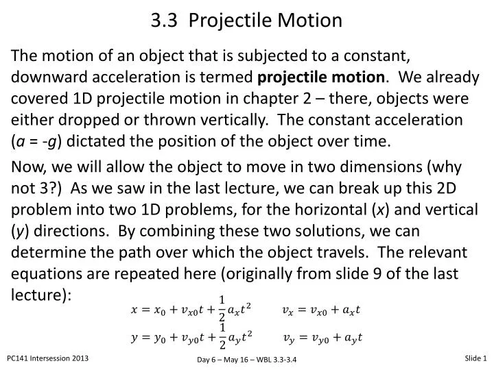
3.3 Projectile Motion The motion of an object that is subjected to a constant, downward acceleration is termed projectile motion. We already covered 1D projectile motion in chapter 2 – there, objects were either dropped or thrown vertically. The constant acceleration (a = -g)dictated the position of the object over time. Now, we will allow the object to move in two dimensions (why not 3?) As we saw in the last lecture, we can break up this 2D problem into two 1D problems, for the horizontal (x) and vertical (y) directions. By combining these two solutions, we can determine the path over which the object travels. The relevant equations are repeated here (originally from slide 9 of the last lecture):
3.3 Projectile Motion Since the acceleration is downward, we can state that ay= -g and ax= 0. In other words, the horizontal motion is defined by zero acceleration (constant velocity), and the vertical motion is defined by constant acceleration. Horizontal Projection We begin with the case that the projectile’s initial velocity is horizontal. Since there is no horizontal acceleration, we can say that at all times, vx= vx0. Furthermore, this means that the horizontal position is a linear function of time: x = x0 + vx0t.
3.3 Projectile Motion While the projectile is traveling at a constant horizontal velocity, it is also traveling vertically. However, since there is a non-zero vertical acceleration, the vertical velocity is not constant. This causes the projectile to move in a curved path. The figure to the right shows two objects that are released at the same time – the red ball is dropped from rest while the yellow ball is projected horizontally. At any given time, both balls have dropped the same vertical distance. The vertical motion and horizontal motion are “uncoupled” (they don’t depend on each other). Both balls will land at exactly the same time.
3.3 Projectile Motion Projections at Arbitrary Angles The most general case of projectile motion is one in which the object is launched at an arbitrary angle θ relative to the horizontal. It has initial velocity components and .
3.3 Projectile Motion Since there is no horizontal acceleration, the x-component of velocity is constant. It will always equal . However, since there is vertical acceleration (ay = -g), the y-component of velocity varies with time, according to the 1D kinematics equations from chapter 2. In summary, As the figure on the previous slide indicates, the projectile will land with the same speed at which it was launched (although the vertical component of velocity will be reversed in sign). The angle at which it lands will be . This assumes that the landing height is the same as the launch height.
3.3 Projectile Motion If we place the origin at the launch point, then . In this case, the kinematic equations from chapter 2 (with ax = 0) produce In the case that the launch point is not the origin, we can simply replace with and with .
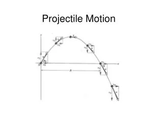
3.3 Projectile Motion At this point, the text proclaims that “the curve described by these equations…is called a parabola”. Let’s prove that, since it’s not too hard. The previous equations describe x and y as functions of time. However, the figure on slide 4 shows the trajectory of the projectile, which is actually y as a function of x. Nothing is plotted as a function of time (although the position of the object is shown at 7 particular times during the projectile’s flight). To find y(x), we follow two steps: • Invert the x(t) equation to find t(x) • Substitute this into the y(t) equation to convert it to y(x)
3.3 Projectile Motion Following these steps, we find that And therefore Since are all constants, this function has the form which describes a parabola. Again, if the launch position is rather than (0,0), then we simply replace with and with .
Problem #1: Thrown Football WBL LP 3.9 (modified)
3.3 Projectile Motion A very important aspect of projectile motion is the range,R. This is the horizontal distance traveled when the object returns to its original height. The text describes one method of calculating R on p. 83. Here’s another method: by the definition of R, we’re simply looking for the value of x that results in y = 0. One solution is x = 0. However, this just reproduces the launch point. The more useful solution (which requires a bit of algebra and trigonometry) is The range is a function of the launch conditions as well as the magnitude of the gravitational acceleration (g).
3.3 Projectile Motion Now that we know where a projectile will land, it’s natural to ask: is there an optimum launch angle, which will maximize the range? This is obviously quite important in areas such as athletics and artillery fire. Since , if are constant, we can maximize R by maximizing sin 2. This occurs when , and produces
3.3 Projectile Motion In real life, projectiles are subject to air resistance. Incorporating this factor into an analysis of projectile motion is beyond the scope of PC141. If we were to do so, we would find that the optimum launch angle is somewhat less than . For the rest of this course, unless otherwise specified, assume that there is no air resistance.
Problem #2: Kicked Football The figure shows three paths for a football kicked from ground level. Note that all three paths have the same maximum height, but they have different ranges. Rank them in terms of time of flight (longest to shortest) Rank them in terms of initial vertical velocity component (fastest to slowest) Rank them in terms of initial horizontal velocity component (fastest to slowest) Rank them in terms of initial speed (fastest to slowest) Solution: In class
Problem #3: Long Jump In the 1991 World Track and Field Championships, Mike Powell jumped a distance of 8.95 m (breaking a 23-year-old world record by 5 cm). Assume that Powell’s speed on takeoff was 9.5 m/s. How much less was Powell’s range than the maximum possible range for an object launched at the same speed? What is the greatest source of the discrepancy in a)? What would Powell’s distance have been if he had run just a bit faster, with a speed on takeoff of 9.6 m/s (and the same initial angle as before)? Solution: In class
Problem #4: Flying Fish Fish use various techniques to avoid their predators. The California flying fish propels itself out of the water using its tail, at a typical speed of 30 km/h. If this fish left the water at a 45° angle, how far could it travel through the air? Suppose a nearby fisherman measured the distance as 180 m. How could this be explained? Solution: In class
Problem #5: Volleyball A volleyball court is 18.0 m long (end-to-end) , and the top of the net is 2.24 m above the ground (for women’s competition). Using a jump serve, a player strikes the ball at a point that is 3.00 m above the ground, and 8.00 m away from the net. The initial motion of the ball is horizontal. What is the minimum initial velocity if the ball is to clear the net? What is the maximum initial velocity of the ball is to land in bounds on the other side of the net? Solution: In class
3.4 Relative Velocity In chapter 2, we learned that an object’s position is measured relative to an arbitrary origin. As it turns out, any measurement of an object’s velocity is also dependent on the velocity of the observer. As an example, you may think you’re jogging at 5 m/s, but that’s only relative to a reference frame that is pinned to the Earth. Since the Earth is spinning about its axis, and rotating about the sun (which itself is moving relative to the center of the Milky Way galaxy), an alien who is observing you from far away would claim that you’re moving much faster than 5 m/s. In most cases in PC141, the “pinned to the Earth” reference frame is appropriate. However, sometimes we need to deal with velocities relative to each other.
3.4 Relative Velocity Relative velocities are indicated using multiple subscripts. For example, means “velocity of object B relative to observer A”. When the velocities of A and B are measured relative to a common reference frame, then (note the order of the subscripts). In the figure, velocities are shown relative to the Earth. Since A is stationary, we have and
3.4 Relative Velocity In this figure, there is no physical distinction in comparison to the last figure. However, now we want to measure velocities relative to car B (that is, relative to a reference frame that is pinned to car B rather than to the Earth). In this case, we need to find and . Using the same subscript ordering as before, we have - In other words, the driver of car B sees car A as traveling at 90 km/h in the negative direction. Similarly, - More examples can be found on pp. 90-92 of the text.
3.4 Relative Velocity Sometimes, the various velocities in a physical problem do not have a common reference point. Here’s a 1D example from the text (the results are still valid in 2D and 3D). Consider a moving walkway (w) in an airport that moves relative to the ground (g) with velocity . A passenger (p) walks on it with a velocity relative to the walkway of . The passenger’s velocity relative to the ground is Again, the ordering of the subscripts is important. The “inner” subscripts in the sum are identical, and the “outer” subscripts are those which appear in the left side. Page 90 of the text contains numerical examples.
Problem #6: Oncoming Traffic WBL LP 3.11
Problem #7: Airplane with Crosswind WBL Ex 3.84 (modified) An airplane is flying at 150 km/h (its speed in still air) in a direction such that with a wind of 60 km/h blowing from east to west, the airplane travels in a straight line southward. What must be the plane’s heading (direction) for it to fly directly south? If the plane has to go 200 km in the southward direction, how long does it take? Solution: In class