Download

1 / 47
470 likes | 558 Views
Explore the design choices and challenges in sensor networks, focusing on TinyOS, Tiny sensor nodes, energy efficiency, resource minimization, and fault tolerance in operating systems. Learn key lessons and innovative approaches for optimal performance and cost savings in sensor deployments.

E N D
Design Choices for Sensor Networks SanthoshPrabhu, Mohammad Ahmad Advanced Distributed Systems CS 525
Tiny, self contained computers • Sensors to collect data • Used in coordinated sensing and monitoring • Deployed in inhospitable/unsafe environments • Relatively low cost, so somewhat expendable Sensor Nodes
Example Hardware • Size • Golem Dust: 11.7 cu. mm • MICA motes: Few inches • Everything on one chip: micro-everything • processor, transceiver, battery, sensors, memory, bus • MICA: 4 MHz, 40 Kbps, 4 KB SRAM / 512 KB Serial Flash, lasts 7 days at full blast on 2 x AA batteries Slide from Indy’s talk on Feb-6
Energy Efficiency • Limited Resources • Fault Tolerance Design Challenges:
} • In: • Operating Systems (TinyOS) • Communication (Directed Diffusion) • Energy Efficiency • Limited Resources • Fault Tolerance Design Challenges: (Today’s Topics)
TinyOS • Operating system designed for embedded devices • Emerged from UC Berkeley in 2000 • Sensor research was beginning • Developed in nesC (a new C dialect) • Currently averages 25,000 downloads a year • Worldwide community of developers and users
Overview • Key design goals of TinyOS • Resource minimization • Bug prevention • What lessons can be drawn from the experience of the TinyOS development?
Resource minimization • TinyOS software should use as few hardware resources as possible • Trade off runtime flexibility for smaller code and data • Computationally efficient • Minimizing cycle counts and wake time • Require little state • Minimize RAM • Tight code • Minimize ROM
Microcontroller specification TI MSP430 Microcontrollers
Why resource minimization is important? • Energy • Parts with more hardware draw more power both when awake and when asleep • ‘every bit transmitted brings a sensor node one moment closer to death’ • Cost • Becomes significant for large scale use • A $6 cut in price for 100,000 units leads to $600,000 in savings
Prevention principle • In-field debugging of sensor networks in notoriously difficult • Unknown input • Unreliable wireless communication • Limited resources make traditional debugging techniques (logging) unsuitable • TinyOS should be structured to make it harder to write bugs
Approach • Pushed dynamic runtime operations into static compile time ones • Evolved language primitives and abstractions to achieve this goal • Allowed for near optimal RAM usage and dependable software systems
ROM and RAM Allocation • ROM minimization • Inlining and dead code elimination • RAM minimization • Goal for TinyOS: Want system calls to require as little RAM as possible • Goal for traditional OS: Want to make system calls as fast as possible
Example: RAM Minimization • Timer service • 32 bit timer requires 10 bytes of state • Pre-1.0 • Initial implementation maintained a linked list of timer structures • Required an additional 2 bytes for the pointer (20% overhead) • V-1.0 • Allocate fixed array of timer structures • nesC introduced ‘unique’ as a way of distinguishing between the timer structures • Problem: Overprovisioning • V-1.1 • Introduced ‘uniqueCount’ which returns the number of times unique has been called with a particular string • Allowed for minimum allocation of resources for timer structures • Allocate exactly how much is required
Isolation • TinyOS 1.x had poor isolation between components – shared memory pools • Example: Packet transmission • Components share queues so its possible for a badly behaving component to starve others • Need to consider that any operation might fail, increasing ROM and RAM use • Concluded that shared memory pools violated the prevention principle and required more resources
Static Virtualization • Static Virtualization • Each component can declare a logical instance of a service • Each component’s interaction to an underlying shared resource is completely independent • Enables software to use an OS service isolated from all other users • Compile time certainty
What lessons can be drawn from the experience of TinyOS development ?
Initial Users • How to get the initial users • Promote use internally (Click modular router) • Provide grants to work on the system • NEST project • Made using TinyOS a requirement for grants • Advantages • Moved project beyond UC Berkeley • Disadvantages • Focusing on growth within research community led to more focus on technical complexity
LanguageCo-design • Advantages: • Flexibility to handle new problems • nesC’s language features contributed to prevention and minimization • Disadvantages • Barrier to entry • Making it easier to solve hard problems made it harder to solve easy ones • Staffing • Suggested Solution • Split design and evolution efforts
Modular Structure • Components are key to TinyOS design • Advantages: • Structured so that it is easy to modify and extend • Easy to verify small components • Disadvantages: • Difficult to understand system for the first time • Tiny pieces of functionality spread across files with different levels of indirection • Overkill! • Solution • Restructure as things stabilize
Conclusion • Very successful as an academic project • Averages 25,000 downloads a year • Significant impact outside academia • Where is missed out • Simple sensing applications • Do it yourself • Platform for the ‘internet of things’ • Connect sensors to the internet • Contiki
The pervasive concerns of energy/resource usage and fault tolerance • Limited control over the topology – Nodes are usually scattered randomly • Mobility of nodes – Nodes may be moved around • Real-time response requirement Concerns
Most approaches borrowed from the MANET world • Table driven (Proactive) Protocols: • Each node keeps a list of destinations and the corresponding routes • Example: DSDV • On-demand (Reactive) Protocols: • Routes established when there is data to be sent • Example: AODV The first step: Routing Algorithms
MANET Algorithms are not the way to go • Table driven (Proactive) Protocols: • Periodic message exchanges • Unnecessary memory usage • On-demand (Reactive) Protocols: • Route setup required before transmitting data • They all separate communication from application The first step: Routing Algorithms
Can we use in-network aggregation to minimize communication overhead? • Can we achieve better fault tolerance with minimal reconfiguration? • How can application knowledge help us design better protocols? Efficient routing protocols are good, but can we do better?
Data centric data dissemination paradigm • Named data in attribute-value pair format • Operator queries transformed into interests - Data requested by sending interests • Interests are diffused toward the nodes in a specific region • Upon interest reception, nodes collect data via their sensors and return it along the reverse path • Intermediate nodes might perform data aggregation Directed Diffusion:
Multi-path delivery for robustness • Application specific path selection • Adaptive choice of transmission rates • Aggregation reduces communication overhead • Nodes can be anonymous – Only local interactions, so no global identifiers required Directed Diffusion: Benefits
Specification of a data-collection task, identified by attribute-value pairs • Any query is translated into an interest • type = wheeled vehicle // type of data to be collected • Interval=20ms //how frequently data needs to be sent • duration=10s //how long to monitor • rect=[-100,100,200,400] //area where monitoring is to be done Directed Diffusion: Interests
A node initiating a task (sink) injects interests into the network • Interests propagate by • flooding • geographic routing • cache-based routing • Nodes receiving a new interest caches the interest and creates a gradient entry for the interest to the sender • Specifies: • The node to which data matching the interest should be sent • Data rate (intervals between data messages) • Duration (Time at which gradient expires) Directed Diffusion: Interest Propagation
Possibly multiple gradients per interest at node (when interest received from multiple neighbors) • Deleted after timeout duration • Can be updated by new interest messages • Interest deleted if no more gradients remain • Initial Gradients – Low data rate, exploratory Directed Diffusion: Gradients
Nodes in the specified region set up sensors • Data collected at highest data rate among all gradients • Sends event description to neighbors with for whom gradients exist • type = wheeled vehicle • instance = truck • location = [125,220] • intensity = 0.6 • confidence = 0.85 • timestamp = 01:20:40 Directed Diffusion: Data Propagation
Received data checked against a cache • New data cached and forwarded • Drop duplicates (prevents loops in forwarding) • Down-conversion: Data forwarded no faster than required Directed Diffusion: Data Propagation
Collect more information along better paths • Done by raising data rate with chosen neighbors • type = wheeled vehicle type = wheeled vehicle • Interval=20ms Interval=5ms • duration=10s duration=10s • rect=[-100,100,200,400] rect=[-100,100,200,400] • Options: • Neighbor that sent data first • Every neighbor that sent data recently • Neighbors that consistently send new data • Choice determines what kind of path is favored Directed Diffusion: Reinforcement
Truncate undesirable paths • Done by: • Timeouts • Explicit negative reinforcement (low data rate interest) • Options: • Consistently old events • Ranking neighbors on number of new events received • Tradeoff between energy efficiency and fault tolerance Directed Diffusion: Negative Reinforcement
Helps in local repairs • Removes loops Directed Diffusion: Reinforcement X
Comparing Directed Diffusion with the alternatives: • Flooding data from source to sink • Omniscient Multicast: End to end communication along shortest path • ns-2 simulation • Increasing network size (in steps of 50) • Average node density kept constant Directed Diffusion: Experiments
Directed Diffusion: Energy use Average Energy (Joules/Node/Received Pkt) Network Size • Diffusion compared to flooding, Omniscient Multicast • Reduced communication due to aggregation
Directed Diffusion: Delay Delay(secs) Network Size • No global knowledge • But paths comparable to Omniscient Multicast • Empirical path selection with local decisions works well • Flooding suffers from collisions
Directed Diffusion: Failure Tolerance Average Energy (Joules/Node/Received Pkt) Network Size • Lower energy consumption under more failures!! • Unnecessary redundancy due to conservative reinforcement
Discussion Points • Static virtualization does away with shared memory pools. Doesn’t this lead to resource wastage? • Could traditional protocols benefit from named data? (Question from CS525 Spring 2013) • Content Delivery Networks • Would rebuilding TinyOS be worth it?
Discussion Points • Picking the right data rate – A tradeoff between energy efficiency and event detection • Congestion free network assumed • Can aggregation slow down communication? • Complete knowledge should help in minimizing bugs anyway • Does caching in diffusion conflict with the idea with the RAM usage minimization?