Optimization of Source Modules
220 likes | 356 Views
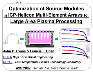
Optimization of Source Modules in ICP-Helicon Multi-Element Arrays for Large Area Plasma Processing. John D. Evans & Francis F. Chen UCLA Dept of Electrical Engineering LTPTL - Low Temperature Plasma Technology Laboratory. AVS 2002 , Denver, Co, November 4, 2002.

Optimization of Source Modules
E N D
Presentation Transcript
Optimization of Source Modules in ICP-Helicon Multi-Element Arrays for Large Area Plasma Processing John D. Evans & Francis F. Chen UCLADept of Electrical Engineering LTPTL- Low Temperature Plasma Technology Laboratory AVS 2002, Denver, Co, November 4, 2002
Conceptual multitube m=0 helicon source for large area processing
COIL COIL UCLA One-tube configuration using large-area Bo-field coils and radially scannable Langmuir probes Single source tube with individual solenoidal Bo
B m=-1 m=+1 B m=+1 m=-1 UCLA Schematic proof of low-field Helicon mode; RH-t-III antenna Helicity pitch sense B up (down) launches m=+1 up (down) Np and VL enhanced in region that m=+1 mode propagates towards
Sense of helicity “LH” “RH” Experimental evidence: Half-helical antennas launch m = +1 Helicon mode from source tube when “low field peak” is present. RH 1/2-helical antenna Dependence of N(B) on thedirection of B reverses when the sense of the helicity of the antenna is reversed; thus it is m = +1 helicon mode LH 1/2-helical antenna
Verification of Low-field Helicon Excitation Low-field “peak” in N vs B plot Dependence of occurrence of peak on B-field direction Dependence of N vs B on B-direction reverses with antenna helicity
Low-field peak increases, broadens and shifts to higher B at higher Po.
UCLA Left Hand (LH) Helical Antenna Nomenclature Defined Lant = Physical length of active antenna element lant = Antenna Wavelength - pitch ofhelical straps l Half Helix
Radial Np profiles for 3 RH-helical antennas 1kW, 13.56MHz, 15mT Ar, 150G, z=3cm, next slide Same antenna length, but different “antenna wavelengths” Top: double-helix; Middle: full-helix; Bottom: half-helix Wider profiles observed in “B-down” configuration in all cases Most total downstream Np produced in full-helix case More total downstream Np produced in “B-down” case m=1 helicon mode enhances profile width as well as Np
Radial Np profiles for 3 RH-helical antennas 1kW, 13.56MHz, 15mT Ar, 150G, z=3cm, next slide Same antenna length, but different “antenna wavelengths” Top: double-helix; Middle: full-helix; Bottom: half-helix Wider profiles observed in “B-down” configuration in all cases Most total downstream Np produced in full-helix case More total downstream Np produced in “B-down” case m=1 helicon mode enhances profile width as well as Np
UCLA 1kW, 15mT, 150G Half-helical m = +1 antenna Lant = 10cm, lant = 20cm Langmuir Probe @ z = 3 cm below mouth of source tube
l UCLA Full-helical m = +1 antenna Lant = 10cm, lant = 10cm Langmuir Probe @ z = 3 cm below mouth of source tube
UCLA Double-helical m = +1 antenna Lant = 10cm, lant = 5 cm Langmuir Probe @ z = 3 cm below mouth of source tube
l UCLA 1kW, 10mT Ar, 13.56MHz, Lant =10cm = lant, z=3cm, 150G
M = 0 radial profiles 4 equispaced source tubes, Enough for uniform plasma? YES, for axial distance z > 10cm from source tubes
Pyrex antenna Schematic of multi-turn loop “m=0” source element
“1,2,4,6” 3 3 4 4 2 2 1 1 5 5 7 7 6 6 Numerical label convention: 7 tube source, aerial view “w,x,y,z” = Antennas # W, X, Y, Z “ON”, others “OFF” “1,2,4,5”
“1,2,4,5” “1,2,4,6” 3 4 3 4 2 1 5 2 1 5 6 7 7 6
“1,2,4,5” 3 4 2 1 5 7 6 Np radial nonuniformity vs axial distance z from source tubes Broad/flat cannot be explained by streaming of plasma along B-lines and normal diffusion
CONCLUSIONS 4 equispaced source tubes good enough, due to Helicon-enhanced uniformity Multitube concept appears to be applicable to arbitrarily large area.