Multilevel Modeling
Multilevel Modeling. Soc 543 Fall 2004. Presentation overview. What is multilevel modeling? Problems with not using multilevel models Benefits of using multilevel models Basic multilevel model Variation one: person and time Variation two: person, time, and space. Multilevel models.

Multilevel Modeling
E N D
Presentation Transcript
Multilevel Modeling Soc 543 Fall 2004
Presentation overview • What is multilevel modeling? • Problems with not using multilevel models • Benefits of using multilevel models • Basic multilevel model • Variation one: person and time • Variation two: person, time, and space
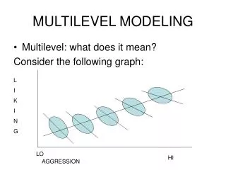
Multilevel models • Units of analysis are nested within higher-level units of analysis • Students within schools • Observations with person
Problems without MLM • If we ignore higher-level units of analysis => cannot account for context (individualistic approach) • If we ignore individual-level observation and rely on higher-level units of analysis, we may commit ecological fallacy (aggregated data approach) • Without explicit modeling, sampling errors at second level may be large =>unreliable slopes • Homoscedasticity and no serial correlation assumptions of OLS are violated (an efficiency problem). • No distinction between parameter and sampling variances
Advantages of MLM • Cross-level comparisons • Controls for level differences
General MLM • Example: Raudenbush and Bryk, 1986 • Dependent variable: • Continuous • Observed
General MLM • High school and beyond (HSB) survey • 10,231 students from 82 Catholic and 94 public schools • Dependent variable: standardized math achievement score • Independent variable: SES
General MLM Variability among schools • Level one: within schools mathij = b0j + b1j (SESij - SES•j) + rij
General MLM Variability among schools • Level two: between schools b0j = g00 + u0j b1j = g10 + u1j
General MLM Variability among schools • Combined model mathij = g00 + u0j + g10(SESij - SES•j) + u1j(SESij - SES•j) + rij = g00 + g10(SESij - SES•j) + u0j + vij (Easy interpretation given the “centering” parameterization)
General MLM Variability among schools • Combined model mathij = 100.74 + 4.52(SESij - SES•j) + u0j + vij • There is a positive relation between SES and math score
General MLM Variability among schools • Results: math score means • school means are different • 90% of the variance is parameter variance • 10% is sampling variance • Results: math score-SES relation • school relations are different • 35% is parameter variance (this requires additional assumption and analysis) • 65% is sampling variance
General MLM Covariates at level 2 Level one: within schools mathij = b0j + b1j (SESij - SES•j) + rij
General MLM Covariates at level 2 • Level two: between schools b0j = g00 + g01sectj+ u0j b1j = g10 + g11sectj+ u1j
General MLM Covariates at level 2 • Combined model: mathij = g00 + g01sectj + g10 (SESij - SES•j) + g11sectj(SESij - SES•j) + rij + vj
General MLM • Combined model: mathij = 98.37 + 5.06sectj + 6.23(SESij - SES•j) - 3.86sectj(SESij - SES•j) + rij + vj
General MLM Variability as a function of sector • Results: math score means • 80.7% is parameter variance • differences in school means is not entirely accounted for by sector • Results: SES-math score relation • 9.7% is parameter variance • differences in school SES-math score relation may be accounted for by sector
General MLM Sector effects • Cannot say that previous relations are causal – may be selection effects • Use example of homework to explain sector differences
General MLM Sector effects • Results: • school SES is strongly related to mean math score, but SES composition accounts for Catholic difference • schools with lower SES had weaker SES-math score relation than higher SES schools
General MLM Sector effects • Results: • variation in SES-math score relation may be accounted for by school SES • variation in mean math score is not entirely accounted for by school SES
MLM with person and time • When observations are repeated for the same units, we also have a nested structure. • Examining within-person changes over time – growth curve analysis. • Growth curves may be similar across persons within a class. • Example: Muthén and Muthén • Dependent variable: categorical, latent
Muthen and Muthen • NLSY • N=7326 (part 1); N=924 (part 2); N=922 (part 3); N=1225 (part 4) • Dependent variables: antisocial behavior (excluding alcohol use) during past year, in 17 dichotomous items; alcohol use during past year, in 22 dichotomous items
MLM with person and time • Part 1: latent class determination by latent class analysis and factor analysis • It’s a cross-sectional analysis of baseline data in 1980. • It found 4 latent classes.
MLM with person and time • Part 2: growth curve determination by latent class growth curve analysis and growth mixture modeling • It uses longitudinal information. • Different growth curves are allowed and estimated for different latent classes. • Growth mixture modeling is a generalization of latent class growth analysis, in allowing growth variance within class • GMM yields a 4-class solution.
MLM with person and time • Part 3: latent class relation to growth curve model by general growth mixture modeling (GGMM) • What’s new is to the ability to predict a categorical outcome variable from latent classes. • The example also illustrates how covariates that predict membership in classes (Table 4).
MLM with person and time • Part 4: latent class relation to growth curve model by GGMM • Multiple (2) latent class variables. • The first one comes from Part 1; the second one comes from Part 2. • It bridges the two component parts, asking how the first class membership affects membership in the second class scheme.
MLM with person, time & space • Example: Axinn and Yabiku • Dependent variable: dichotomous, observed • Hazard model with event history
MLM with person, time & space • Chitwan Valley Family Study (CVFS) • 171 neighborhoods (5-15 household cluster) • Dependent variable: initiated contraception to terminate childbearing
MLM with person, time & space Age 0 Age 12 Birth of 1st child Contraceptive use or end of observation Time-invariant childhood community context Time-varying contemporary community context Time-invariant early life nonfamily experiences Time-varying contemporary nonfamily experiences
MLM with person, time & space • Level one: Logit(ptij) = b0j + b1Cj+ b2Xij +b3Djt + b4Zijt C: time-invariant community var. D: time-variant community var. X: time-invariant personal var. Z: time-variant personal var. (Note that there is no interaction across levels)
Multi-level Hazard Models • There is a general problem with non-linear multi-level models. • Unbiasedness breaks down. • Special attention needs to be paid to estimation of hazard models in a multi-level setting. • See Barber et al (2000).