Download
1 / 86
860 likes | 872 Views
Explore the regulatory control laye.r structure and key decision points for plantwide control systems. Learn Sigurd’s rules for flow control cascade and how to establish consistency in inventory control. Understand the importance of the Throughput Manipulator (TPM) and its impact on production rates.

E N D
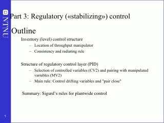
Part 3: Regulatory («stabilizing») control Outline Inventory (level) controlstructure • Location ofthroughput manipulator • Consistency and radiatingrule Structureofregulatorycontrollayer (PID) • Selectionofcontrolled variables (CV2) and pairingwithmanipulated variables (MV2) • Main rule: Control drifting variables and "pair close" Summary: Sigurd’srules for plantwidecontrol
Example flow control cascade Process: F = k(z)*sqrt(dp) Japanize slide. Linearize in two points. P-control Find closed-loop tf from Fs to F.
Procedure • Skogestad procedure for control structure design I Top Down • Step S1: Define operational objective (cost) and constraints • Step S2: Identify degrees of freedom and optimize operation for disturbances • Step S3: Implementation of optimal operation • What to control ? (primary CV’s) • Active constraints • Self-optimizing variables for unconstrained, c=Hy • Step S4:Where set the production rate? (Inventory control) II Bottom Up • Step S5: Regulatory control: What more to control (secondary CV’s) ? • Step S6: Supervisory control • Step S7: Real-time optimization
Step S4. Where set production rate? • Very important decision that determines the structure of the rest of the inventory control system! • May also have important economic implications • Link between Top-down (economics) and Bottom-up (stabilization) parts • Inventory control is the most important part of stabilizing control • “Throughput manipulator” (TPM) = MV for controlling throughput (production rate, network flow) • Where set the production rate = Where locate the TPM? • Traditionally: At the feed • For maximum production (with small backoff): At the bottleneck
TPM and link to inventory control • Liquid inventory: Level control (LC) • Sometimes pressure control (PC) • Gas inventory: Pressure control (PC) • Component inventory: Composition control (CC, XC, AC)
Production rate set at inlet :Inventory control in direction of flow* TPM * Required to get “local-consistent” inventory control
Production rate set at outlet:Inventory control opposite flow* TPM * Required to get “local-consistent” inventory control
Production rate set inside process* TPM * Required to get “local-consistent” inventory control
General: “Need radiating inventory control around TPM” (Georgakis)
Consistency of inventory control Consistency (required property): An inventory control system is said to be consistentif the steady-state mass balances (total, components and phases) are satisfied for any part of the process, including the individual units and the overall plant.
QUIZ 1 CONSISTENT?
Local-consistency rule Rule 1. Local-consistency requires that 1. The total inventory (mass) of any part of the process must be locally regulated by its in- or outflows, which implies that at least one flow in or out of any part of the process must depend on the inventory inside that part of the process. 2. For systems with several components, the inventory of each component of any part of the process must be locally regulated by its in- or outflows or by chemical reaction. 3. For systems with several phases, the inventory of each phase of any part of the process must be locally regulated by its in- or outflows or by phase transition. Proof: Mass balances Note: Without the word “local” one gets the more general consistency rule
QUIZ 1 CONSISTENT? Rule (March 2017): Controlling pressure at inlet or outlet gives indirect flow control (because of pressure boundary condition)
Local concistency requirement -> “Radiation rule “(Georgakis)
Flow split: May give extra DOF TPM TPM Split: Extra DOF (FC) Flash: No extra DOF
Example: Separator controlAlternative TPM locations Compressor could be replaced by valve if p1>pG
Alt.2 Alt.1 Alt.4 Alt.3 Similar to original but NOT CONSISTENT (PC not direction of flow) Rule: Setting in-pressure p0 sets inflow = TPM at inlet Setting out-pressure pG sets outflow = TPM at outlet (left two cases)
Example: Solid oxide fuel cell xCH4,s CC PC CH4 CH4 + H2O = CO + 3H2 CO + H2O = CO2 + H2 2H2 + O2- → 2H2O + 2e- H2O (in ratio with CH4 feed to reduce C and CO formation) e- TPM = current I [A] = disturbance O2- Solid oxide electrolyte O2 + 4e- → 2O2- Air (excess O2) PC TC Ts = 1070 K (active constraint)
LOCATION OF SENSORS • Location flow sensor (before or after valve or pump): Does not matter from consistency point of view • Locate to get best flow measurement • Before pump: Beware of cavitation • After pump: Beware of noisy measurement • Location of pressure sensor (before or after valve, pump or compressor): Important from consistency point of view
PC PC FC FC FC PC PC PC FC FC For each of the five structures; Where is the TPM? Is it feasible?
PC FC FC FC PC PC FC PC FT PT Same sensor location as case 3. Can you control both flow and temperature using valves 2 and 3, Valves 3 and 4? Some more. For each of the five structures; Where is the TPM? Is it feasible?
FC PC PC FC FC PC PC Solution according to radiation rule TPM NO PC FC YES TPM NO TPM FC YES (it does not matter where the flow is measured; the valve determines the location of the TPM) TPM YES TPM Note: Can never control pressure at ends (upstream first control valve or downstream last valve)!
PC FC FC TPM NO FC PC NO. New Rule: Another controller cannot cross the TPM, Not even with a PC TPM PC NO, cannot cross TPM TPM FC PC NO TPM FT PT No, but OK if we use valve 4 for PC Some more. For each of the five structures; Where is the TPM? Is it feasible?
Where should we place TPM? • TPM = MV used to control throughput • Traditionally: TPM = Main feed valve (or pump/compressor) • Gives inventory control “in direction of flow” Consider moving TPM if: • There is an important CV that could otherwise not be well controlled • Dynamic reasons • Special case: Max. production important: Locate TPM at process bottleneck* ! • TPM can then be used to achieve tight bottleneck control (= achieve max. production) • Economics: Max. production is very favorable in “sellers marked” • If placing it at the feed may yield infeasible operation (“overfeeding”) • If “snowballing” is a problem (accumulation in recycle loop), then consider placing TPM inside recycle loop BUT: Avoid a variable that may (optimally) saturate as TPM (unless it is at bottleneck) • Reason: To keep controlling CV=throughput, we would need to reconfigure (move TPM)** *Bottleneck: Last constraint to become active as we increase throughput -> TPM must be used for bottleneck control **Sigurd’s general pairing rule (to reduce need for reassigning loops): “Pair MV that may (optimally) saturate with CV that may be given up”
Example TPM: Two distillation columns • See end of part 1
Often optimal: Locate TPM at bottleneck! • "A bottleneck is a unit where we reach a constraints which makes further increase in throughput infeasible" • If feed is cheap and available: Located TPM at bottleneck (dynamic reasons) • If the flow for some time is not at its maximum through the bottleneck, then this loss can never be recovered.
Alt.1. Feedrate controls bottleneck flow (“long loop”…): Fmax FC Fmax Alt. 3: Reconfigure all upstream inventory loops: Fmax Single-loop alternatives for bottleneck control Bottleneck. Want max flow here Traditional: Manual control of feed rate TPM TPM Alt. 2: Feedrate controls lost task (another “long loop”…): TPM TPM
May move TPM to inside recycle loop to avoid snowballing Example: Eastman esterification process Alcohol recycle Reach max mass transfer rate: R increases sharply (“snowballing”) Ester product Alcohol + water + extractive agent (e)
Final improvement: Located “at” bottleneck + TPM is inside “snowballing” loop Follows Luyben’s law 1 to avoid snowballing(modified): “Avoid having all streams in a recycle system on inventory control”
CASE STUDY: Recycle plant(Luyben, Yu, etc.)Part 1 -3 Recycle of unreacted A (+ some B) 5 Feed of A 4 1 2 Assume constant reactor temperature. Given feedrate F0 and column pressure: 3 Dynamic DOFs: Nm = 5 Column levels: N0y = 2 Steady-state DOFs: N0 = 5 - 2 = 3 Product (98.5% B)
Part 1: Economics (Given feed) Recycle plant: Optimal operation mT 1 remaining unconstrained degree of freedom, CV=?
J=V as a function of reflux L Optimum = Nominal point With fixed active constraints: Mr = 2800 kmol (max), xB= 1.5% A (max)
Control of recycle plant:Conventional structure (“Two-point”: CV=xD) LC TPM LC xD XC XC xB LC Control active constraints (Mr=max and xB=0.015) + xD
Luyben law no. 1 (to avoid snowballing): “Fix a stream in the recycle loop” (CV=F or D)
Luyben rule: CV=D (constant) LC LC XC LC
“Brute force” loss evaluation:Disturbance in F0 Luyben rule: Conventional Loss with nominally optimal setpoints for Mr, xB and c
Loss evaluation: Implementation error Luyben rule: Loss with nominally optimal setpoints for Mr, xB and c
Conclusion: Control of recycle plant Active constraint Mr = Mrmax Self-optimizing L/F constant: Easier than “two-point” control Assumption: Minimize energy (V) Active constraint xB = xBmin
Modified Luyben’s law to avoid snowballing • Luyben law no. 1 (“Plantwide process control”, 1998, pp. 57): “A stream somewhere in all recycle loops must be flow controlled” • Luybenruleis OK dynamically (short time scale), • BUT economically (steady-state): Recycle should increase with throughput • Modified Luyben’s law 1 (by Sigurd): “Consider moving the TPM inside the recycle loop”
PC NOTE: There are actually two recycles • One through the reactor (D or F) • One through the column (L) • One flow inside both recycle loops: V • Alt.6: TPM=V if we want to break both recycle loops! TC
PC Alt. 6 TPM = V LC LC L XC TC F TPM XC LC Simulations (to be done) confirm This is the best! L and F for composition control: OK!
PC Alt. 7 What about keeping V constant?(in addition to having another TPM) LC TPM L LC TC F0 F V XC LC With feedrate F0 fixed (TPM) L for compostioncontrol in bottom (xB) Topcompositionfloating NO! Never control cost J=V
Reactor-recycle process: Want to maximize feedrate: reach bottleneck in column Bottleneck: max. vapor rate in column TPM
Reactor-recycle process with max. feedrateAlt.A: Feedrate controls bottleneck flow Bottleneck: max. vapor rate in column TPM Vs FC Vmax V Vmax-Vs=Back-off = Loss Get “long loop”: Need back-off in V
Reactor-recycle process with max. feedrate:Alt. BMove TPM to bottleneck (MAX). Use feedrate for lost task (xB) Bottleneck: max. vapor rate in column MAX TPM =Alt.6 TPM Get “long loop”: May need back-off in xB instead…
Reactor-recycle process with max. feedrate:Alt. C: Best economically: Move TPM to bottleneck (MAX) + Reconfigure upstream loops LC MAX TPM OK, but reconfiguration undesirable… =Alt.6 TPM
Reactor-recycle process:Alt.C’: Move TPM + reconfigure (permanently!) LC CC TPM F0s =Alt.6 TPM For cases with given feedrate: Get “long loop” but no associated loss