Download
1 / 25
250 likes | 376 Views
Informed Search II. CIS 391 Fall 2008. Outline. PART I Informed = use problem-specific knowledge Best-first search and its variants A * - Optimal Search using Knowledge Proof of Optimality of A * A * for maneuvering AI agents in games Heuristic functions? How to invent them PART II

E N D
Informed Search II CIS 391 Fall 2008
Outline PART I • Informed = use problem-specific knowledge • Best-first search and its variants • A* - Optimal Search using Knowledge • Proof of Optimality of A* • A* for maneuvering AI agents in games • Heuristic functions? • How to invent them PART II • Local search and optimization • Hill climbing, local beam search, genetic algorithms,… • Local search in continuous spaces • Online search agents
Optimality of A* (intuitive) • Lemma: A* expands nodes in order of increasing fvalue • Gradually adds "f-contours" of nodes • Contour i has all nodes with f=fi, where fi < fi+1
Optimality of A* using Tree-Search I (proof) • Suppose some suboptimal goal G2has been generated and is in the fringe. Let n be an unexpanded node in the fringe such that n is on a shortest path to an optimal goal G. • g(G2) > g(G) since G2 is suboptimal • f(G2) = g(G2) since h(G2) = 0 • f(G) = g(G) since h(G) = 0 • f(G2) > f(G) from 1,2,3
Optimality of A* using Tree-Search II (proof) • Suppose some suboptimal goal G2has been generated and is in thefringe. Let n be an unexpanded node in the fringe such that n is on ashortest path to an optimal goal G. • f(G2) > f(G) repeated • h*(n) h(n) since h is admissible, and therefore optimistic • g(n) + h*(n) g(n) + h(n) from 5 • g(n) + h*(n) f(n) substituting definition of f • f(G) f(n) from definitions of f and h* (think about it!) • f(G2) >f(n) from 4 & 8 So A* will never select G2 for expansion
A* search, evaluation • Completeness: YES • Since bands of increasing f are added • As long as b is finite • (guaranteeing that there aren’t infinitely many nodes with f<f(G) )
A* search, evaluation • Completeness: YES • Time complexity: • Number of nodes expanded is still exponential in the length of the solution.
A* search, evaluation • Completeness: YES • Time complexity: (exponential with path length) • Space complexity: • It keeps all generated nodes in memory • Hence space is the major problem not time
A* search, evaluation • Completeness: YES • Time complexity: (exponential with path length) • Space complexity:(all nodes are stored) • Optimality: YES • Cannot expand fi+1 until fi is finished. • A* expands all nodes with f(n)< f(G) • A* expands one node with f(n)=f(G) • A* expands no nodes with f(n)>f(G) Also optimally efficient (not including ties)
Proof of Lemma: Consistency • A heuristic is consistent if • If h is consistent, we have i.e. f(n) is nondecreasing along any path. Theorem: if h(n) is consistent, A* using Graph-Search is optimal Cost of getting from n to n’ by any action a
Search for AI Simulation Graphics from http://theory.stanford.edu/~amitp/GameProgramming/ (A great site for practical AI & game Programming)
Best-First Search • Yellow: nodes with high h(n) • Black: nodes with low h(n)
Dijkstra’s Algorithm • Pink: Starting Point • Blue: Goal • Teal: Scanned squares • Darker: Closer to starting point…
A* Algorithm • Yellow: examined nodes with high h(n) • Blue: examined nodes with high g(n)
Dijkstra’s Algorithm Dijkstra's algorithm works harder but is guaranteed to find a shortest path
A* Algorithm A* finds a path as good as Dijkstra's algorithm found, but is much more efficient…
Heuristic functions • For the 8-puzzle • Avg. solution cost is about 22 steps • (branching factor ≤ 3) • Exhaustive search to depth 22: 3.1 x 10¹⁰ states • A good heuristic function can reduce the search process
Admissible heuristics E.g., for the 8-puzzle: • hoop(n) = number of out of place tiles • hmd(n) = total Manhattan distance (i.e., # of moves from desired location of each tile) • hoop(S) = ? • hmd(S) = ?
Admissible heuristics E.g., for the 8-puzzle: • hoop(n) = number of out of place tiles • hmd(n) = total Manhattan distance (i.e., # of moves from desired location of each tile) • hoop(S) = ? 8 • hmd(S) = ? 3+1+2+2+2+3+3+2 = 18
Relaxed problems • A problem with fewer restrictions on the actions is called a relaxed problem • The cost of an optimal solution to a relaxed problem is an admissible heuristic for the original problem • If the rules of the 8-puzzle are relaxed so that a tile can move anywhere, then hoop(n) gives the shortest solution • If the rules are relaxed so that a tile can move to any adjacent square, then hmd(n) gives the shortest solution
Defining Heuristics: h(n) • Cost of an exact solution to a relaxed problem (fewer restrictions on operator) • Constraints on Full Problem: A tile can move from square A to square B ifA is adjacent to Band B is blank. • Constraints on relaxed problems: • A tile can move from square A to square B ifA is adjacent to B. (hmd) • A tile can move from square A to square B if B is blank. • A tile can move from square A to square B. (hoop)
Dominance • If h2(n) ≥ h1(n)for all n (both admissible) • then h2dominates h1 • So h2is optimistic, but more accurate than h1 • h2is therefore better for search • Typical search costs (average number of nodes expanded): • d=12 Iterative Deepening Search = 3,644,035 nodes A*(hoop) = 227 nodes A*(hmd) = 73 nodes • d=24 IDS = too many nodes A*(hoop) = 39,135 nodes A*(hmd) = 1,641 nodes
Iterative Deepening A* and beyond Beyond our scope: • Iterative Deepening A* • Recursive best first search (incorporates A* idea, despite name) • Memory Bounded A* • Simplified Memory Bounded A* - R&N say the best algorithm to use in practice, but not described here at all. • (see pp. 101-104 if you’re interested)