Download
1 / 61
620 likes | 755 Views
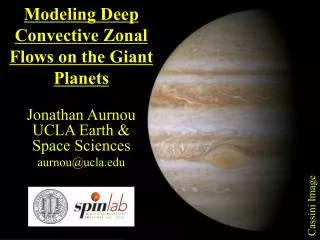
Modeling Deep Convective Zonal Flows on the Giant Planets. Jonathan Aurnou UCLA Earth & Space Sciences aurnou@ucla.edu. Cassini Image. Acknowledgements. Moritz Heimpel University of Alberta mheimpel@phys.ualberta.ca. Johannes Wicht Max Plank Institute for Aeronomy wicht@linmpi.mpg.de.

E N D
Modeling Deep Convective Zonal Flows on the Giant Planets Jonathan Aurnou UCLA Earth & Space Sciences aurnou@ucla.edu Cassini Image
Acknowledgements • Moritz Heimpel • University of Alberta • mheimpel@phys.ualberta.ca • Johannes Wicht • Max Plank Institute for Aeronomy • wicht@linmpi.mpg.de
Today’s Seminar • A new model of zonal flow dynamics on the Giant Planets • Observations • Shallow Layer Models • Deep Convection Models • Yano’s Shallow Model • Deep Jovian Convection Model • Deep Convection Model for the Ice Giants
Jovian Zonal Wind Observations • Jovian winds movie from Cassini: Cassini Website
Jovian Zonal Wind Observations • Polar winds movie from Cassini: A. Vasavada
Jovian Wind Observations • East-west velocities w/r/t B-field frame • Powerful prograde equatorial jet • Smaller wavelength higher latitude jets • Fine scale jets near poles • Net prograde winds
Giant Planet Atmospheres • Deep atmospheric shell aspect ratios (c = ri/ro) • Jupiter: c = 0.75 ~ 0.95, Saturn: c = 0.4 ~ 0.8
Thermal Emission • Jupiter and Saturn’s thermal emission ~ twice solar insolation • Neptune’s ~ 3 times solar insolation • Uranus is anomalous • Zonal winds could be due to either shallow or deep energy sources
Thermal Emission • Jupiter and Saturn’s thermal emission ~ twice solar insolation • Neptune’s ~ 3 times solar insolation • Uranus is anomalous • Zonal winds could be due to either shallow or deep energy sources
Zonal Wind Models • Shallow layer models • Deep Convection models • Both models are able to generate aspects of the observed zonal winds
Shallow Layer Models • Turbulent flow on a rotating spherical surface of radius ro • No convection • Simulates dynamics of outer weather layer
Turbulence • 3D Turbulence: Energy cascades from injection scale eddies down to dissipation scale eddies • 2D Turbulence: “Inverse Cascade” of energy; eddies tend to grow to domain size
Potential Vorticity Conservation • In an inviscid shallow layer, potential vorticity (PV), q, is conserved:
+y -y b - Plane Approximation • Taylor expand planetary vorticity, f : • On a spherical surface • Ambient PV gradient: Increasing PV towards poles
Potential Vorticity Conservation • For inviscid 2D flow on the b-plane: • For sufficiently large L :
Shallow Layer Rhines Length • Rhines, JFM, 1975 • Rhines scale, LR, where curvature effects truncate 2D inverse cascade: • At LR, turbulenteddies cease to grow • Energy gets transferred into zonal motions • Scale of zonal jets
Shallow Layer Models • Shallow layer turbulence evolves into: • Large-scale zonal flows • Alternating bands • Coherent vortices Cho & Polvani, Science, 1996
Shallow Layer Models • Shallow layer turbulence evolves into: • Large-scale zonal flows • Alternating bands • Coherent vortices Saturn Latitude Jupiter Equatorial jets are westward Cho & Polvani, Science, 1996
Shallow Layer Models • 2D turbulence evolves into Rhines scale zonal jets • Shallow layer b-effect • Potential vorticity increases towards poles • Gives retrograde equatorial jets • Iacono et al., 1999; Vasavada & Showman, 2005
Deep Layer Models • Busse, 1976 • Deep spherical shell dynamics • Multiple jets require nested cylinders of convection columns • And even then… Busse, Icarus, 1976
Rotating Spherical Shell Dynamics • Geostrophic quasi-2D dynamics • Axial flow structures • Tangent cylinder (TC) flow barrier
The Topographicb-effect • PV Conservation in a deep shell: • PV gradient: Increasing PV towards equator, opposite the shallow layer case
The Topographicb-effect • PV conservation on the topographic b-plane • Induced local vorticity causes eastward drift Equatorial plane, viewed from above
The Topographicb-effect • PV conservation on spherical boundary causes latitudinally-varying drift rate & tilted columns Equatorial plane, viewed from above
Reynolds Stresses Equatorial plane, viewed from above
Tangent Cylinder Quasi-laminar Deep Convection Models North pole view of equatorial plane isotherms Outer boundary heat flux from 20oN lat Aurnou & Olson, GRL, 2001
Shallow Layer: Imposed turbulence on a spherical shell Increasing PV with latitude Retrograde equatorial jet Higher latitude Rhines scale jets Deep Convection: Quasi-laminar, QG convection Decreasing PV with latitude Prograde equatorial jet No higher latitude alternating jets Shallow vs. Deep Model Comparison
Yano’s Shallow Layer Model Yano et al., Nature (2003)
Yano’s Shallow Layer Model • Yano et al., 2003 • 2D shallow layer turbulence model • Chooses a different function for b • Full spheretopographic b parameter • Opposite sign as shallow layer b • Simulates geostrophic turbulence in a sphere using the 2D shallow layer equations
Yano’s Shallow Layer Model • Prograde equatorial jet • Broad Rhines scale high latitude jets Solid Lines: Model Dashed Lines: Observed Yano et al., Nature, 2003
Yano’s Shallow Layer Model • Sign of b controls direction of equatorial jet • Broad high latitude jets do not resemble Jovian observations • Suggests that Rhines scale jets can form from quasigeostrophic (~2D) convective turbulence in a deep 3D model
4. New Deep Convection Model Heimpel, Aurnou & Wicht, Nature, 438: 193-196 (2005)
Spherical Shell Rhines Scale Outside TC Inside TC Tangent Cylinder (Scaling discontinuity across TC)
Spherical Shell Rhines Scale • The Rhines scale is discontinuous across the tangent cylinder • In thin shells: • Thebt parameter becomes larger inside the tangent cylinder • LR becomes smaller
Geometric Scaling Function Heimpel & Aurnou, 2006
Zonal Winds vs. Radius Ratio Tests Heimpel & Aurnou, 2006
Recent Jovian Interior Models Guillot et al., 2004
New Deep Convection Model • Rapidly-rotating, turbulent convection • Thin shell geometry (c = 0.90; 7000 km deep)
c=0.35 Rotating Convection Studies • Christensen, 2002 • Zonal flow from fully-developed, quasigeostrophic turbulence • Asymptotic regime Ro 0.01 0.1 1 Ra* Christensen, JFM, 2002
New Deep Convection Model • Solve Navier-Stokes equation • Energy equation • Boussinesq (incompressible) fluid • Wicht’s MagIC2 spectral transform code • Spherical harmonics in lat. & long. • Difficulties in resolving flows near poles • Chebyschev in radius • Courant time-step using grid representation
New Deep Convection Model • Input Parameters: • Ra = 1.67 x 10¹⁰ • E = 3 x 10⁻⁶ • Pr = 0.1 • Ra* = RaE2/Pr = 0.15 • ri/ro = c = 0.90 • Resolution • Lmax = 512, grid: f 768, q 192, r 65 • Hyperdiffusion and 8-fold f -symmetry • Output Parameters: • Re ~ 5 x 10⁴ • Ro ~ 0.01
c=0.90 Model Results Azimuthal Velocity Temperature
Zonal Wind Profiles c=0.90 Model Jupiter
Jupiter Model The “Tuning” Question • We have chosen • the radius ratio • The lowest Ekman number feasible • i.e., Fastest rotation rate • A Rayleigh number such that our peakRo is similar to Jupiter’s • Close to asymptotic regime of Christensen, 2002
3D Spherical Shell Rhines Scale • “Regional” 3D shell Rhines scale c=0.90 Model Jupiter
New Deep Convection Model • Quasigeostrophic convective turbulence in a relatively thin spherical shell • Generates coexisting prograde equatorial jets & alternating higher latitude jets • Model (& Jovian observations) follows Rhines scaling for a 3D shell • Scaling discontinuity across the tangent cylinder • Smaller-scale jets inside tangent cylinder
Following Work 1 • Why do we need “regional” Rhines fits? • Expensive to test with full 3D models • 2D quasigeostrophic mechanical models • 2D quasigeostrophic convection models