Download
1 / 56
560 likes | 724 Views
Annika Schomburg, Christoph Schraff. Assimilating satellite cloud information with an Ensemble Kalman Filter at the convective scale. EUMETSAT fellow day, 17 March 2014, Darmstadt. Motivation: Weather situation 23 October 2012.

E N D
Annika Schomburg, Christoph Schraff Assimilating satellite cloud information with an Ensemble Kalman Filter at the convective scale EUMETSAT fellow day, 17 March 2014, Darmstadt
Motivation: Weather situation 23 October 2012 12 UTC synoptic situation: stable high pressure system over central Europe
Motivation: Weather situation 23 October 2012 12 UTC synoptic situation: low stratus clouds over Germany Satellite cloud type classification
Motivation: Verification for 23 October 2012 12 hour forecast from 0:00 UTC Low cloud cover: COSMO-DE versus satellite Total cloud cover: COSMO-DE versus synop T2m: COSMO-DE minus synop Green: hits;black: misses red: false alarms, blue: no obs Courtesy of K. Stephan
Motivation Main motivation: improvecloudcoversimulationoflowstratusclouds in stable wintertime high-pressuresystems • May also beusefulfor frontal systemorconvectivesituations • Ifconvectivecloudsarecapturedbetterwhiledeveloping, convectiveprecipitationmaybeimproved
Outline • Introduction • The COSMO model • The ensemble Kalman filter • Clouddata • Assimilation approach • Assimilated variables andmodelequivalents • Results • Single observationexperiments • Cyclingexperiment • Forecast • Conclusionandoutlook • Future application
Outline • Introduction • The COSMO model • The ensemble Kalman filter • Clouddata • Assimilation approach • Assimilated variables andmodelequivalents • Results • Single observationexperiments • Cyclingexperiment • Forecast • Conclusionandoutlook • Future application
The COSMO model • COSMO-DE : • Limited-area short-rangenumerical modelweatherpredictionmodel • x 2.8 km / 50 vertical layers • Explicit deep convection • New data assimilation system : Implementation of the Ensemble Kalman Filter
Outline • Introduction • The COSMO model • The ensemble Kalman filter • Clouddata • Assimilation approach • Assimilated variables andmodelequivalents • Results • Single observationexperiments • Cyclingexperiment • Forecast • Conclusionandoutlook • Future application
Local Ensemble Transform Kalman Filter Observation errors R Analysis perturbations: linear combination of background perturbations LETKF OBS-FG OBS-FG OBS-FG OBS-FG Background error covariance Obs First guess ensemble members are weighted according to their departure from the observations.
Local Ensemble Transform Kalman Filter Observation errors R Analysis perturbations: linear combination of background perturbations LETKF OBS-FG OBS-FG OBS-FG OBS-FG Background error covariance Obs • Local: the linear combinationisfitted in a localregion • - observationhave a spatially limited influenceregion • Transform: mostcomputationsarecarried out in ensemblespace computationallyefficient • Implementation after Hunt et al., 2007 11
Local Ensemble Transform Kalman Filter Observation errors R Analysis perturbations: linear combination of background perturbations LETKF OBS-FG OBS-FG OBS-FG OBS-FG Background error covariance Obs Additional: one deterministic run: Kalman gainmatrixfrom LETKF
Outline • Introduction • The COSMO model • The ensemble Kalman filter • Clouddata • Assimilation approach • Assimilated variables andmodelequivalents • Results • Single observationexperiments • Cyclingexperiment • Forecast • Conclusionandoutlook • Future application
Which observations? Forshortrange limited-areamodels: geostationarysatellitedata: Meteosat-SEVIRI (Δx ~ 5km overcentral Europe, Δt=15 min) Here: Assimilation ofNWC-SAF cloud top height Source: EUMETSAT Cloud top height Retrieval algorithm needs temperature and humidity profile information from a NWP model cloud top height might be at wrong height if temperature-profile in NWP model is not simulated correctly! use also radiosonde information where available 1 2 3 4 5 6 7 8 9 10 11 12 13 Height [km]
“Cloud analysis“: Combine satellite & radiosonde information Radiosonde relative humidity Satellite cloud top • Use nearby radiosondes within the same cloud typeto correct • (or approve) cloud top height from satellite cloud height retrieval Radiosondes: coverage Satellite cloud type
Combine satellite & radiosonde information: data availability flag • Use temporal and spatial distance of radiosonde for weighting: • Also use data availability flag for observation error specification: γ 1.0 0.8 0.6 0.4 0.2
Combine satellite & radiosonde information Cloud top height Satellite cloud product Cloudanalysis Obs-error [m]
Outline • Introduction • The COSMO model • The ensemble Kalman filter • Clouddata • Assimilation approach • Assimilated variables andmodelequivalents • Results • Single observationexperiments • Cyclingexperiment • Forecast • Conclusionandoutlook • Future application
relative humidity height of model level k = 1 Z [km] Determine the model equivalent cloud top model profile k1 k2 Cloud top CTHobs k3 k4 k5 • (make sure to choose the top of the detected cloud) • use y=CTHobsH(x)=hk • and y=RHobs=1H(x)=RHk(relative humidity over water/ice depending on temperature) • as 2 separate variables assimilated by LETKF RH [%] • Avoid strong penalizing of members which are dry at CTHobs but have a cloud or even only high humidity close to CTHobs search in a vertical range hmaxaround CTHobs for a ‘best fitting’ model level k, i.e. with minimum ‘distance’ d:
Example: 17 Nov 2011, 6:00 UTCObservations and model equivalents „Cloud top height“ Observation Model RH model level k
Determinemodelequivalent: cloudfreepixels Z [km] What information can we assimilate for pixels which are observed to be cloudfree? 12 „no high cloud“ • assimilate cloud fraction CLC = 0 separately • for high, medium, low clouds • model equivalent: • maximum CLC within vertical range 9 „no mid-level cloud“ 6 3 „no low cloud“ CLC
Example: 17 Nov 2011, 6:00 UTC • COSMO cloud cover where observations “cloudfree” Low clouds (oktas) Mid-level clouds (oktas) High clouds (oktas)
Schematic illustration of approach cloudy obs = 1 = 0 cloud-free obs
Outline • Introduction • The COSMO model • The ensemble Kalman filter • Clouddata • Assimilation approach • Assimilated variables andmodelequivalents • Results • Single observationexperiments • Cyclingexperiment • Forecast • Conclusionandoutlook • Future application
„Single observation“ experiment • Analysis for 17 November 2011, 6:00 UTC (no cycling) • Each column is affected by only one satellite observation • Objective: • Understand in detail what the filter does with such special observation types • Does it work at all? • Detailed evaluation of effect on atmospheric profiles • Sensitivity to settings
Single-observation experiments: missed cloud event • 1 analysis step, 17 Nov. 2011, 6 UTC (wintertime low stratus) vertical profiles relative humidity cloud cover cloud water cloud ice observed cloud top 3 lines in one colour indicate ensemble mean and mean +/- spread
Single-observation experiments: missed cloud event Cross section of analysis increments for ensemble mean relative humidity [%] specific water content [g/kg] observed cloud top observation location
Deterministic run First guess Analysis Relative humidity Cloud cover Cloud water Cloud ice Observed cloud top Humidity at cloud layer is increased in deterministic run
Missed cloud case: Effect on temperature profile temperature profile [K] (mean +/- spread) first guess analysis observed cloud top • LETKF introduces inversion due to RH T cross correlations • in first guess ensemble perturbations
Single-observation experiments: False alarm cloud assimilated quantity: cloud fraction (= 0) vertical profiles relative humidity cloud cover cloud water cloud ice observed cloud top 3 lines on one colour indicate ensemble mean and mean +/- spread
Increment cross section ensemble mean Observation location Observed cloud top
FG ANA FG ANA Single-observation experiments: False alarm cloud • Observation cloudfree assimilated quantity: cloud fraction (= 0) Observation minus model histogram over ensemble members low cloud cover fraction [octa] mid-level cloud cover fraction [octa] LETKF decreases erroneous cloud cover despite very non-Gaussian distributions
Outline • Introduction • The COSMO model • The ensemble Kalman filter • Clouddata • Assimilation approach • Assimilated variables andmodelequivalents • Results • Single observationexperiments • Cyclingexperiment • Forecast • Conclusionandoutlook • Future application
Sensitivityexperiment: Data thinning • 1-hourly cycling over 21 hours with 40 members • 13 Nov., 21UTC – 14 Nov. 2011, 18UTC • wintertime low stratus • Thinning: • 8 km • 14 km • 20 km
Sensitivity experiment: Data density RH at observed cloud top Cloud cover • Comparing experiments with different data density: • 8 km • 14 km • 20km Low clouds Mid-level clouds High clouds Solid: 8km Dashed: 14km Dotted: 20km RMSE Bias (OBS-FG) Mean squared error for low/medium/high cloud cover averaged over all observed cloud free pixels RMSE and bias averaged over all cloudy observations Forcloudypixelsbestresultsareobtainedfor a 14 km thinningdistance, forcloud-freeobservationsnoclearconclusion
Sensitivity experiment: Data density • Comparingexperimentswith different datadensity: • 8 km • 14 km • 20km • The spreadforthe 8km thinningexperimentislowerthantheothertwo, thedifference in spreadbetweenthe 14 and 20 experimentsissmaller. • Ensemble isunderdispersive, but thereisnosignof a furtherreductionofthespreadduringthecycling RMSE Spread
Comparisoncyclingexperiment: onlyconventional vs conventional + clouddata • 1-hourly cycling over 21 hours with 40 members • 13 Nov., 21UTC – 14 Nov. 2011, 18UTC • Wintertime low stratus • Thinning: 14 km
Comparison “only conventional“ versus “conventional + cloud obs" Time series of first guess errors, averaged over cloudy obs locations RH (relative humidity) at observed cloud top assimilation of conventional obs only assimilation of conventional + cloud obs RMSE Bias (OBS-FG) • Cloud assimilation reduces RH (1-hour forecast) errors
Comparison of cycled experiments Total cloud cover of first guess fields after 20 hours of cycling conventional + cloud conventional only satellite obs Satellite cloud top height 12 Nov 2011 17:00 UTC
Cycled assimilation of dense observations Time series of first guess errors, averaged over cloud-free obs locations (errors are due to false alarm clouds) mean square error of cloud fraction [octa] low clouds High clouds • False alarm clouds reduced through cloud data assimilation
Comparison “only conventional“ versus “conventional + cloud obs" ‘false alarm’ cloud cover (after 20 hrs cycling) high clouds mid-level clouds low clouds conventional obs only [octa] conventional + cloud
Outline • Introduction • The COSMO model • The ensemble Kalman filter • Clouddata • Assimilation approach • Assimilated variables andmodelequivalents • Results • Single observationexperiments • Cyclingexperiment • Forecast • Conclusionandoutlook • Future application
Comparisonforecastexperiment: onlyconventional vs conventional + clouddata • 24h deterministic forecast based on analysis of two experiments (after 12 hours of cycling) • 14 Nov., 9UTC – 15 Nov. 2011, 9UTC • Wintertime low stratus
Comparison of free forecast: time series of errors RH (relative humidity) at observed cloud top averaged over all cloudy observations Mean squared error averaged over all cloud-free observations • The forecastofcloudcharacteristicscanbeimprovedthroughtheassimilationofthecloudinformation RMSE Bias (Obs-Model) Low clouds Mid-level clouds High clouds Conventional + cloud data Only conventional data
Verification against independent measurements Conventional + cloud data Only conventional data Errors for SEVIRI infrared brightness temperatures (model values computed with RTTOV) RMSE Bias (Obs-Model) RMSE issmallerforfirst 16 hoursofforecastforcloudexperiment, biasvaries
Verification against independent measurements: SEVIRI brightness temperature errors Only CONV experiment CONV+CLOUD experiment • Also the high cloudsaresimulatedbetter in thecloudexperiment 14 Nov 2011, 18 UTC Cloud top height
Outline • Introduction • The COSMO model • The ensemble Kalman filter • Clouddata • Assimilation approach • Assimilated variables andmodelequivalents • Results • Single observationexperiments • Cyclingexperiment • Forecast • Conclusionandoutlook • Future application
Conclusions • Use of (SEVIRI-based) cloud observations in LETKF: • Tends to introduce humidity / cloud where it should (+ temperature inversion) • Tends to reduce ‘false-alarm’ clouds • Despite non-Gaussian pdf’s • Long-lasting free forecast impact for a stable wintertime high pressure system
Next steps • Evaluate impact on other variables (temperature, wind) • Other cases (e.g. convective) • Also work on direct SEVIRI radiance assimilation • Revision on QJRMS article on single observation experiments, publish second article on full cycling and forecasts results • Application in renewable energy project EWeLiNE…
Outline • Introduction • The COSMO model • The ensemble Kalman filter • Clouddata • Assimilation approach • Assimilated variables andmodelequivalents • Results • Single observationexperiments • Cyclingexperiment • Forecast • Conclusionandoutlook • Future application