Download
1 / 30
300 likes | 458 Views
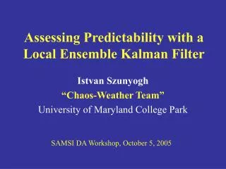
Assessing a Local Ensemble Kalman Filter. Istvan Szunyogh “Chaos-Weather Team” University of Maryland College Park. IPAM DA Workshop, UCLA, February 22-25, 2005. System Components.

E N D
Assessing a Local Ensemble Kalman Filter Istvan Szunyogh “Chaos-Weather Team” University of Maryland College Park IPAM DA Workshop, UCLA, February 22-25, 2005
System Components • Data assimilation scheme: Local Ensemble (Transform) Kalman Filter (Ott et al. 2002, 2004; Hunt 2005) implemented by Eric Kostelich (ASU) and I. Sz. • Model: Operational Global Forecast System (GFS) of the National Centers for Environmental Prediction/National Weather Service • Model Resolution: T62 (~150 km) in the horizontal directions and 28 vertical level dimension of the state vector:1,137,024; dimension of the grid space (analysis space): 2,544,768]
WARNING!!!!! All results shown in this presentation were obtained for the perfect model scenario
Why a Perfect Model? • Easier to find bugs in the code • To expose weaknesses of the scheme (model errors cannot be blamed for unexpected bad results) • To establish a reference needed to assess the effects of model errors • To learn more about the dynamics of the model (predictability, dimensionality, etc.)
Local Ensemble Kalman FilterIllustration on a two dimensional grid • The state estimate is updated at the center grid point • The background state is considered only from a local region (yellow dots) • All observations are considered from the local region (purple diamonds)
Base Experiment • Number of ensemble members: 40 • Local regions: 7x7xV grid point cubes; V=1, 3, 5, 7 • Variance Inflation: Multiplicative, uniform 4% (needed to compensate for the loss of variance due to nonlinearities and sampling errors) • Observations: 2000 vertical sounding of wind, temperature, and surface pressure
Depth of Local Cubes Lower stratosphere Upper troposphere Dimension of Local State Vector ~1,700 Mid-troposphere Lower troposphere
Time evolution of errors surface pressure Observational error Rms analysis error analysis cycle (time) The error settles at a similarly rapid speed for all variables 15-days (60 cycles) is a safe upper bound estimate for the transient
Zonal-Mean Analysis Error(45-day mean)The analysis errors are much smaller than the observational errors Temperature u-wind The “largest” errors: deep convection (maximum CAPE), polar regions
Time-Mean Analysis Error45-day average Temperature 60 kPa u-wind 30 kPa NH Extratropics N-America Euro-Asia Africa Tropics S-America Australia SH Extratropics The figures confirm the conclusions drawn based on zonal means
E-dimension A local measure of complexity Illustration in 2D model grid space A spatio-temporally changing scalar value is assigned to each grid point Based on the eigenvalues of the ensemble based estimate of the local covariance matrix: Introduced by Patil, Hunt et al. (2001) Studied in details by Oczkowski et al (2005) Complexity: E-dimension 1 Number of Ensemble Members-1 The more unevenly distributed the variance in the ensemble space, the lower the E-dimension
Explained (Background) Error Variance Illustration for a rank-2 covariance matrix (3-member ensemble) True state Eigenvector 1 Explained Variance: be2/ b2 b Projection on the plane of the eigenvectors be Background mean Eigenvector 2 A perfect explained variance of 1 implies that the space of uncertainties is correctly captured by the ensemble, but it does not guarantee that the distribution of the variance within that space is correctly represented by the ensemble
E-dimension, Explained Variance, Analysis Error • Background ensemble perturbations span the space, where corrections to the estimate of the state can be made => E-dimension characterizes the distribution of variance between distinct state space directions, EV measures the potential for a correction • A correction is realized, when the difference between the observation and the background mean has a projection on the subspace that contributes to the explained variance • Low explained variance or low E-dimension would be a problem if the error in the resulting state estimate was large
E-Dimension and Explained Variance E-dimension Explained BackgroundVariance The E-dimension and Explained Background Variance seem to be strongly anti-correlated. The E-dimensionsis thehighest, theexplained varianceis thelowest, in the Tropics. Szunyogh et al. (2005)
E-Dimension vs. Explained Variance Low E-dimension always indicates high explained variance Zonal Mean No Averaging E-dimension E-dimension Correlation:-0.91 Correlation:-0.9 Explained Variance Explained Variance High E-dimension always indicates low explained variance Szunyogh et al. (2005)
Sensitivity to the Size of the Local Region: Part I Temperature, Global Error 3x3xV 5x5xV 7x7xV 9x9xV 11x11xV The performance is only modestly sensitive to the local region size best Observational error worst mid-troposphere rms error Szunyogh et al. (2005)
Sensitivity to the Size of the Local Region: Part II u-wind, NH extra-tropics u-wind, Tropics Best: 5x5xV The tropical wind is the most sensitive analysis variable Worst:11x11xV Observational error Szunyogh et al. (2005)
Sensitivity to the Size of the Local Region and the Ensemble Size u-wind, Tropics, 80-member ensemble the5x5xV localization improves only a little with increasing the ensemble size Observational error The 7x7xV localization breaks even with the 5x5xV localization Szunyogh et al. (2005)
Sensitivity to the Number of Observations Wind Error in Tropics Global Temperature Error 500 soundings 1000 soundings 2000 soundings 18048 soundings (All locations) Szunyogh et al. (2005)
E-dimension and Explained Variance (fully observed atmosphere) E-dimension Explained Variance The largest E-dimension did not change The smallest explained variance was reduced by about 0.05 (about 12%) Error reduction in the tropics is about 46% Szunyogh et al. (2005)
Evolution of the Forecast Errors As forecast time increases the extratropical storm track regions become the regions of largest error 45-day mean D. Kuhl et al.
Evolution of the E-dimension The E-dimension rapidly Decreases in the storm Track regions The error growth and the decrease of the E-dimension is closely related D. Kuhl et al.
Evolution of the Explained Variance The explained variance is the largest in the storm track regions and it increases with time Large error growth, low E-dimension, and large explained variance are closely related There seems to exist a ‘local analogue’ to the unstable subspace D. Kuhl et al.
The scatter plots confirm the increasingly close correspondence between low E-dimensionality and high explained variance (improving ensemble performance) E-dimension Explained Variance D. Kuhl et al.
Time Mean Evolution of the Forecast Errors (exponential growth) (linear growth) Curves fitted for First 72 hours The error doubling time in the extratropics is about 35-37 hours D. Kuhl et al.
The effect of Local Patch Size on the Error Growth in the NH Extratropics… is negligible Forecast hour D. Kuhl et al.
The Effect of the Ensemble Size on the Forecast Errors in the NH Extratropics… is negligible Forecast hour D. Kuhl et al.
The Effect of the Number of Observations on the Forecast Errors in the NH Extratropics Forecast hour The slightly larger growth rate for the initially smaller errors indicates the presence of saturation processes D. Kuhl et al.
Conclusions and Challenges • The state-of-the art model shows local low-dimensional behavior.Is it reasonable to assume that the real atmosphere shows a similar behavior?(My guess: yes) • Local low dimensionality helps obtain more accurate estimate of the initial state and more accurate prediction of the forecast uncertainties. • Localization in the physical space seems to be a practical way to apply low dimensional concepts to a very high dimensional system. Is it possible to develop a rigorous theoretical framework to support this phenomenological result? (I have no guess) • On the practical side, the LETKF assimilates an operational observation file (excluding satellite radiances) in 5 minutes
References • Kuhl, D., I. Szunyogh, E. J. Kostelich, G. Gyarmati, D.J. Patil, M. Oczkowski, B. Hunt, E. Kalnay, E. Ott, J. A. Yorke, 2005: Assessing predictability with a Local Ensemble Kalman Filter (to be submitted) • Szunyogh,I, E. J. Kostelich, G. Gyarmati, D. J. Patil, B. R. Hunt, E. Kalnay, E. Ott, and J. A. Yorke, 2005: Assessing a local ensemble Kalman filter: Perfect model experiments with the NCEP global model. Tellus 57A. [in print] • Oczkowski, M.,I. Szunyogh, and D. J. Patil, 2005: Mechanisms for the development of locally low dimensional atmospheric dynamics. J. Atmos. Sci. [in print]. • Ott, E., B. R. Hunt, I. Szunyogh, A. V. Zimin, E. J. Kostelich, M. Corazza, E. Kalnay, D. J. Patil, J. A. Yorke, 2004: A local ensemble Kalman Filter for atmospheric data assimilation.Tellus 56A , 415-428. • Ott, E., B. R. Hunt, I. Szunyogh, A. V. Zimin, E. J. Kostelich, M. Corazza, E. Kalnay, D. J. Patil, and J. A. Yorke, 2004: Estimating the state of large spatio-temporally chaotic systems. Phys. Lett. A., 330, 365-370. • Patil, D. J., B. R. Hunt, E. Kalnay, J. A. Yorke, and E. Ott, 2001: Local low dimensionality of atmospheric dynamics, Phys. Rev. Let., 86, 5878-5881. • Reprints and preprints of papers by our group are available at http://keck2.umd.edu/weather/weather_publications.htm