Download
1 / 23
230 likes | 247 Views
URBP 204 A Class 6. CLASS 5 Normal Distribution Hypothesis Testing Test between means of related groups Test between means of different groups Analysis of Variance (ANOVA) CLASS 6 Tutorial 2

E N D
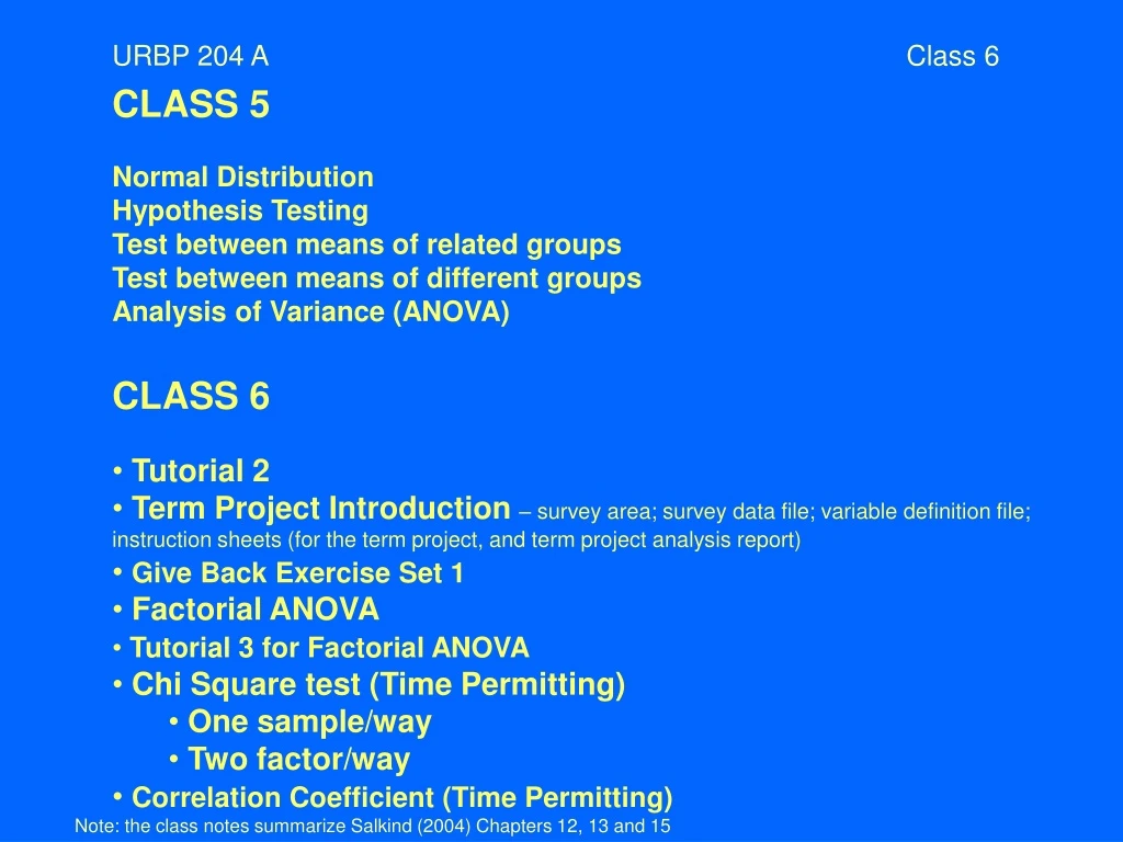
URBP 204 A Class 6 • CLASS 5 • Normal Distribution • Hypothesis Testing • Test between means of related groups • Test between means of different groups • Analysis of Variance (ANOVA) • CLASS 6 • Tutorial 2 • Term Project Introduction – survey area; survey data file; variable definition file; instruction sheets (for the term project, and term project analysis report) • Give Back Exercise Set 1 • Factorial ANOVA • Tutorial 3 for Factorial ANOVA • Chi Square test (Time Permitting) • One sample/way • Two factor/way • Correlation Coefficient (Time Permitting) Note: the class notes summarize Salkind (2004) Chapters 12, 13 and 15
Five Wounds Brookwood Terrace Project One of 20 neighborhood areas identified in the City of San Jose’s Strong Neighborhood Initiative (SNI) FWBT Neighborhood Plan at: http://www.sanjoseca.gov/planning/sni/fivewounds/ Source: http://www.strongneighborhoods.org/strongneighborhoodareas.htm
Five Wounds Brookwood Terrace Project Coyote Creek to its West Lower Silver Creek to North Highway 280 to South Source: http://www.sanjoseca.gov/planning/sni/fivewounds/existing.pdf
Five Wounds Brookwood Terrace Project Population = 20,000 Hispanic – 73.5% (city avg. 32.8%) Asian/ Pacific Islander – 14.5% White/ Non- Hispanic – 7.6% Other – 5% HH Size = 3.5 (city avg. 3.1) Median age lower than the city’s median age of 33.7 years Income Median HH Income - $49,013 (city median HH Income - $73,804) Substantially less than the city median HH Income Education High School Diploma or less (Age greater or equal to 25 years) – 77.3% (city avg. 43.2%) Associate Degree – 18.4% (city avg. 31.5%) Bachelor’ Degree – 7.9% (city avg. 25.3%) Overall less educated than the city-wide population Source: Chapter 2. FWBT Neighborhood Plan.
Five Wounds Brookwood Terrace Project Diverse range of housing types Predominantly SF Source: Chapter 2. FWBT Neighborhood Plan.
Five Wounds Brookwood Terrace Project Census tract numbers 5014.00, 50515.01 and 5015.02 lie fully within the FWBT area while part of census tract number 5036.01 falls within the FWBT area. Source: Mike Reilly, Instructor URBP 179, Fall 2004
Factorial ANOVA Source: Salkind, pg. 215 Note: the class notes summarize Salkind (2004) Chapters 12, 13 and 15
Factorial ANOVA More than 2 factors (independent variables) Education level – low education and high education Gender– male and female 4 groups Low educated male Low educated female High educated female High educated male Dependent variable - minutes biked per day (ratio level variable / continuous variable) Test effect of main independent variables + the interaction term Note: the class notes summarize Salkind (2004) Chapters 12, 13 and 15
Steps for testing 1. Statement of null and research hypothesis H0: Цloweduc = Цhigheduc H0: Цmale = Цfemale H0: Цloweduc X male = Цhigheduc x male = Цhigheduc x female = Цloweduc x female H1: Xloweduc = Xhigheduc H1: Xmale = Xfemale H1: X loweduc X male = X higheduc x male = X higheduc x female = X loweduc x female 2. Set level of risk Level of risk of type I error = 5%, or level of significance = 0.05 3. Selection of appropriate test statistic Choose Factorial ANOVA Note: the class notes summarize Salkind (2004) Chapters 12, 13 and 15
4. Compute the F statistic (Obtained Value) Note: the class notes summarize Salkind (2004) Chapters 12, 13 and 15
5. Determination of the value needed for rejection of null hypothesis (critical value) See table B3, pg. 361-363 Critical value = 3.99 (see Salkind, p.363) 6. Comparison of obtained and critical value Obtained value more extreme than the critical value (F= 111.115, 43.211, and 11.24, are all greater than 3.99) 7. Decision Reject all the three null hypotheses (null hypotheses - there is NO difference between the mean of groups) Probability is less than 5% on any one test of the null hypothesis that the difference between the mean of groups is due to chance alone. Df for numerator: Number of factors-1 = 2-1 =1 Df for denominator: No of observations- no if groups = 68-4 = 64 Note: the class notes summarize Salkind (2004) Chapters 12, 13 and 15
Correlation How the value of one variable changes if the value of the other variable changes. For example, correlation between: Distance from city center and housing price Both variables need to be ratio or interval level. Note: the class notes summarize Salkind (2004) Chapters 12, 13 and 15
Correlation Coefficient Q: How do we know of the correlation is statistically significant? A: Test for significance of the correlation coefficient Source: Salkind, p 230 Note: the class notes summarize Salkind (2004) Chapters 12, 13 and 15
Steps for testing 1. Statement of null and research hypothesis H0: ρxy = 0 No relationship between variables x and y H1: rxy = 0 There is relationship between variables. 2. Set level of risk Level of risk of type I error = 5%, or level of significance = 0.05 3. Selection of appropriate test statistic Choose t-test for the significance of the correlation coefficient Note: the class notes summarize Salkind (2004) Chapters 12, 13 and 15
Coefficient of correlation 4. Obtained value For relationship between Density and distance , r = - 0.74 Density and price, r = 0.81 Distance and price, r = - 0.98 Note: the class notes summarize Salkind (2004) Chapters 12, 13 and 15
5. Determination of the value needed for rejection of null hypothesis (critical value) See table B4, pg. 365 Critical value = 0. 35 (see Salkind, p.363) 6. Comparison of obtained and critical value Obtained value more extreme than the critical value for following relationships: Density and distance , r = - 0.74 Density and price, r = 0.81 Distance and price, r = - 0.98 7. Decision Reject the null hypothesis (null hypothesis - there is NO relationship between the variables). The relationship is not due to chance alone. Degree of freedom = n-2 = 30-2 = 28 Note: the class notes summarize Salkind (2004) Chapters 12, 13 and 15
Non parametric tests • When assumption of normality does not hold (small sample size – less than 30 observations) • Need ordinal or nominal level data. Note: the class notes summarize Salkind (2004) Chapters 12, 13 and 15
One factor/sample chi square Is the distribution of frequencies what you would expect by chance alone? 1. Statement of null and research hypothesis Proportion of occurrence under each category is equal. H1: Proportion of occurrence under each category is not equal. 2. Set level of risk Level of risk of type I error = 5%, or level of significance = 0.05 3. Selection of appropriate test statistic Choose chi square test H0: P1 = P2 = P3 = P4 = P5 P1 = P2 = P3 = P4 = P5
4. Obtained value Note: Should have minimum of 5 observations under each category Note: the class notes summarize Salkind (2004) Chapters 12, 13 and 15
5. Determination of the value needed for rejection of null hypothesis (critical value) See table B5, pg. 367 Critical value = 9.49 (see Salkind, p.363) 6. Comparison of obtained and critical value Obtained value more extreme than the critical value 7. Decision Reject the null hypothesis (null hypothesis - that the distribution of frequencies is equal). Degrees of freedom = number of categories of data – 1 = 5-1 = 4
Two factor/way chi square Explore relationships when both the dependent and the independent variables are nominal or ordinal level, that is “Categorical data” Does the respondents’ age affect their perception about the condition of street lighting? 1. Statement of null and research hypothesis Proportion of occurrence under each category is equal. H1: Proportion of occurrence under each category is not equal. 2. Set level of risk Level of risk of type I error = 5%, or level of significance = 0.05 3. Selection of appropriate test statistic Choose chi square test H0: P1 = P2 = P3 = P4 P1 = P2 = P3 = P4
4. Obtained value Note: Should have minimum of 5 observations under each category Expected Frequency Table Observed Frequency Table 9.75 = (26 x 15) / 40 16.25 = (26 x 25) / 40 5.25 = (14 x 15) / 40 8.75 = (14 x 25) / 40 λ2 = (6-9.75)2 / 9.75 + (20-16.25)2 /16.25 + (5.25-9)2 /5.25 + (8.75-5)2 /8.75 = 6.59
URBP 204 A Class 6 5. Determination of the value needed for rejection of null hypothesis (critical value) See table B5, pg. 367 Critical value = 3.84 (see Salkind, p.363) 6. Comparison of obtained and critical value Obtained value more extreme than the critical value 7. Decision Reject the null hypothesis (null hypothesis - that the distribution of frequencies is equal). Degrees of freedom = (row-1) x (column -1) = (2-1) x (2-1) = 1 x 1 = 1