Section 5 Hypothesis Testing
Section 5 Hypothesis Testing. William Christensen, Ph.D. What is a Hypothesis?. Hypothesis – (in statistics) a claim or statement about a property of a population. Example: a claim that the mean weight of men is greater than 175 lbs.


Section 5 Hypothesis Testing
E N D
Presentation Transcript
Section 5 Hypothesis Testing William Christensen, Ph.D.
What is a Hypothesis? • Hypothesis – (in statistics) a claim or statement about a property of a population. • Example: a claim that the mean weight of men is greater than 175 lbs. • Example: a claim that less than 50% of households in the U.S. have internet access • Example: a claim that annual income levels in St. George have a standard deviation greater than $10,000 • Note: Hypothesis is singular and hypotheses is plural
Hypothesis Testing • In this section you will learn how to test hypotheses related to means, proportions, and standard deviations (or variances) • We use sample data to test claims about population parameters (means, proportions, and standard deviations) • Statistics is all about chance or probability, so our hypothesis tests are always based on some given chance of being right (or wrong) in our answer
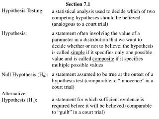
Null & Alternative Hypothesis • Since we do not know in advance what the results are going to be of a hypothesis test, we ALWAYS state the hypothesis in two forms: • H0 (read H-oh or H-zero) is the sign to represent the “Null Hypothesis” and always contains an =, , or sign • H1 (read H-one) is the sign to represent the “Alternative Hypothesis” and always contains the opposite sign (≠, , )
Null & Alternative Hypothesis • Here are examples of all the kinds of hypothesis testing we learn in this section, shown in their proper format: • Hypothesis tests for µ (population Mean) • The claim being tested always determines the value that is used, but in this case we use a value of 100 just as an example
Null & Alternative Hypothesis • Here are examples of all the kinds of hypothesis testing for p (population Proportion) • The claim being tested always determines the value that is used, but in this case we use a value of 0.50 (50%) just as an example. Note that proportions like probabilities must be between 0.0 and 1.0
Null & Alternative Hypothesis • Here are examples of all the kinds of hypothesis testing for σ and σ2 (population Standard Deviation and Variance) • The claim being tested always determines the value that is used, but in this case we use a value of 10 for standard deviation and 100 for variance just as an example
Null & Alternative Hypothesis • You may have noticed that every Null hypothesis contains a “condition of equality” ( =, , or sign) • And that every Alternative hypothesis has the opposite sign as shown in the following table
Doing a Hypothesis Test • The previous slides show every possible combination of Null and Alternative Hypotheses for population Mean, Proportion, and Standard Deviation / Variance. • Now that you know what hypotheses look like, the next step is to learn how to test them.
Doing a Hypothesis Test • It is always the “Null Hypothesis” that is being tested. • If the test “fails” then we reject the Null Hypothesis, or in other words, accept the Alternative Hypothesis • If the test does not fail, then we accept the Null Hypothesis
Doing a Hypothesis Test • Whenever we test hypotheses we are testing a “claim” that has been made • Example: The mean weight of men is greater than 175 lbs. • Whenever possible, it is a good practice to state the claim in terms of the Alternative Hypothesis (not equal, less than, or greater than) rather than the Null Hypothesis (equal, less than or equal, or greater than or equal)
Doing a Hypothesis Test • Here are the steps in doing a hypothesis test • State the Null and Alternative hypotheses • Determine the “Critical Value(s)” and “Critical Region(s)” – this is what we’ll learn next • Calculate the “Test Statistic” and compare it against the Critical Value(s) • If the Test Statistic lies within the Critical Region then reject the null hypothesis (accept the alternative hypothesis) • If the Test Statistic does not lie within the Critical Region then fail to reject the null hypothesis (accept the null hypothesis)
Critical Region(s) and Value(s) • Critical values are the z-scores or x values associated with the standard normal distribution. These values are established based on the level of confidence or alpha value we choose. • Critical regions are bordered by a critical value and include all the area outside (toward the tail). • Whenever we do hypothesis testing we do it based on some level of “confidence” or α (alpha) value • For example, an α = 0.05 represents a 95% confidence level or 95% chance that our answer will be truly correct and a 5% chance that our answer will not be correct. The total area contained in the critical region(s) equals alpha. E.g., if α = 0.05 then the total combined area in these critical regions equals 5% of the total area (0.05/2 = 0.025 on each side) Critical Regions Critical Values
Hypothesis Test: population Mean using large sample (n 30)
Assumptions • When testing claims about population means from large samples we assume the following conditions exist: • The sample is a random sample • The sample is large (n 30)
Critical Value(s) • You actually already know how to find the critical value for hypothesis tests of population Mean using large samples. Remember the Excel function NORMSINV(probability)? It allows us to determine the x value (same as z-score) for a standard normal distribution where we know the area (probability) as measured from the extreme left out to the critical value. • For example, if α = 0.05 (total combined area) then the area from the extreme left to the critical value on the left can be found by NORMSINV(0.025) and the critical value of the right can be found by NORMSINV(0.975) Critical Values Area from left = 0.975 Area from left = 0.025 0.025 0.025
µ Critical Values • Remember the 3 types of null / alternative hypothesis combinations we have: • This is very important in order to properly determine the critical value(s) for nearly ALL HYPOTHESIS TESTS The easy way to remember this is that the sign of the Alternative hypothesis points the direction of the test. A ≠ sign kind of points both ways and represents a two-tail test. A sign points right, and a sign points left.
µ Critical Value Exampleα = 0.05 CV = -1.96 CV = 1.96 Area = α/2 = 0.025 Area = α/2 = 0.025 CV = -1.645 CV = 1.645 Area = α = 0.05 Area = α = 0.05 Notice how critical values for the left-tail are ALWAYS negative and critical values for the right-tail are ALWAYS positive
µ Critical Value Exerciseα = 0.01 CV = -2.576 CV = 2.576 Area = α/2 = 0.005 Area = α/2 = 0.005 Use Excel function NORMSINV to confirm these critical values are correct CV = -2.326 CV = 2.326 Area = α = 0.01 Area = α = 0.01
Test Statistic • A “Test Statistic” is a value we calculate from the sample data • We use the Test Statistic to test our hypothesis by comparing the Test Statistic against the critical value(s) • The following graph shows how the position of the Test Statistic determines whether we accept the Null hypothesis or the Alternative hypothesis If the Test Statistic falls in the critical region(s) then reject the null hypothesis (accept the alternative hypothesis) If the Test Statistic does not fall in the critical region(s) then “fail to reject H0 (accept the null hypothesis)
x - µ Test Statistic= σ n Test Statistic for µ • For large samples, testing claims about population means we calculate the Test Statistic using the following formula (you must remember this one)
x - µ Test Statistic= σ n Test Statistic for µ This is the sample average/mean which we calculate from our sample data We never really know the population mean (µ) but we do have a value included in the hypothesis (e.g., H0: µ=100) and it is this value that we put here – the value from the hypothesis For large samples If we know σ (population std. deviation) then we put it here. However, we usually only have sample data, so we use s (sample std. deviation) here most of the time n is simply the size of our sample. E.g., if our sample consists of 50 men, then n=50
Hypothesis Test Example Itesting a claim about µ from a large sample We generally assume that the average or normal human body temperature is 98.6 degrees F. To test this assumption or claim, data was collected from 106 healthy adults (n = 106). From this sample, the following statistics were obtained. Mean temperature = 98.2o Standard deviation (s) = 0.62o Using an alpha of 0.05 (a 95% confidence level that our solution will be correct, with a 5% chance of being wrong) test the claim that the mean body temperature of all healthy adults is equal to 98.6o.
Hypothesis Test Example Itesting a claim about µ from a large sample • Write out the claim and the hypotheses • The claim is that the mean body temperature of healthy adults is equal to 98.6o or µ = 98.6o • Notice that we are making a claim about the population of all healthy adults, but we only have a sample of 106 adults upon which to test this claim • Thus, the null hypothesis H0: µ = 98.6o • The alternative hypothesis H1: µ ≠ 98.6o • You must be able to read ‘word problems’ and be able to translate them into null and alternative hypotheses
Hypothesis Test Example Itesting a claim about µ from a large sample • Draw a picture of the normal distribution and determine the critical values • Note that the sign of the alternative hypothesis is ≠ so we have a two-tail test Note: since the standard normal distribution is perfectly symmetrical, you can simply take the negative critical value on the left and change it to a positive value for the right side – or go ahead and use NORMSINV again to solve for the right side α = 0.05, α/2 = 0.025 0.4750 0.4750 0.025 0.025 -1.96 1.96 Critical values are determined using Excel NORMSINV
x - µ 98.2 - 98.6 zTS=== - 6.64 s 0.62 n 106 Hypothesis Test Example Itesting a claim about µ from a large sample • Calculate the Test Statistic and form your final conclusion • Remember we were given the following information: • n = 106, s = 0.62o, sample mean = 98.2o, α = 0.05, and our null hypothesis is µ = 98.6o • We can now calculate the Test Statistic using the formula we learned: Note: If the test statistic falls inside the critical values then we always accept the null hypotheses (mean body temperature equals 98.6), and if the test statistic falls outside the critical values we always accept the alternative hypothesis (mean body temperature does not equal 98.6).
0.025 0.025 -1.96 1.96 Critical values determined using Excel NORMSINV Hypothesis Test Example Itesting a claim about µ from a large sample • Calculate the Test Statistic and form your final conclusion We calculated the test statistic zTS = -6.64 CONCLUSION: Accept the alternative hypothesis H1: µ ≠ 98.6o The mean body temperature of healthy adults is not 98.6o F Accept the alternative hypothesis Accept the alternative hypothesis Accept the null hypothesis Test statistic falls outside the critical value
Hypothesis Test Example IItesting a claim about µ from a large sample Men are often accused of channel-surfing (constantly changing channels using the remote control). With this in mind, a study was done to test the claim that, on average, men change channels every 5.00 seconds or less. To investigate this claim, sample data was collected and the following statistics were obtained: n = 80 (80 men were observed) Sample mean = 5.25 seconds standard deviation = 2.50 seconds Use an alpha = 0.10 to test this claim.
Hypothesis Test Example IItesting a claim about µ from a large sample • Write out the claim and the hypotheses • The claim is that men change channels every 5 seconds or less or µ 5.00 seconds • Notice that we are making a claim about the population of all TV-watching men, but we only have a sample of 80 men upon which to test this claim • Thus, the null hypothesis H0: µ 5.0 seconds • The alternative hypothesis H1: µ 5.0 seconds • REMEMBER that the sign for the null hypothesis MUST ALWAYS be =, , or and the sign for the alternative hypothesis is always ≠, , or (the opposite of the null hypothesis)
Hypothesis Test Example IItesting a claim about µ from a large sample • Draw a picture of the normal distribution and determine the critical values • Note that the sign of the alternative hypothesis is so we have a right-tail test Note: since we have a one-tail test to the right, the entire critical region is on the right side and has an area equal to alpha. We can either use NORMSINV(0.10) and change the answer to a positive value, or use NORMSINV(0.90) which will return the same positive value. α = 0.10 0.500 0.400 0.100 1.28 Critical value is determined using Excel NORMSINV
x - µ 5.25 – 5.00 zTS=== 0.89 s 2.50 n 80 Hypothesis Test Example IItesting a claim about µ from a large sample • Calculate the Test Statistic and form your final conclusion • Remember we were given the following information: • n = 80, s = 2.50 seconds, sample mean = 5.25 seconds, α = 0.10, and our null hypothesis is µ 5.0 seconds • We can now calculate the Test Statistic using the formula we learned: Note: If the test statistic falls inside the critical value then we always accept the null hypotheses (men switch channels every 5 seconds or less), and if the test statistic falls outside the critical value we always accept the alternative hypothesis (men wait more than 5 seconds before switching channels).
Hypothesis Test Example IItesting a claim about µ from a large sample • Calculate the Test Statistic and form your final conclusion We calculated the test statistic zTS = 0.89 CONCLUSION: Accept the null hypothesis H0: µ 5.0 seconds Men switch channels every 5 seconds or less Accept the alternative hypothesis Accept the null hypothesis 0.100 Test statistic falls inside the critical value 1.28 Critical value determined using Excel =NORMSINV(0.90)
Hypothesis Test Example IItesting a claim about µ from a large sample • Discussion: Perhaps you noticed in the last exercise that the sample mean was 5.25 seconds and yet we concluded that men change channels every 5 seconds or less. How is this possible? • You must remember that we are talking about probabilities here. We did this problem based on a 90% confidence of being correct (10% chance of being wrong). Therefore, we are not certain about our conclusion, it is just our best estimate based on the info we were given. • We do know that a sample of 80 men does NOT give us exactly the same data as we would have if we knew the channel-surfing habits of all men in our population. Certainly if the mean channel-surfing interval for all men was 5.25 seconds then it would be ridiculous to make any other claim. However, in this case we must make our conclusion about the entire population of men based on our sample of only 80 men. • Since our sample mean of 5.25 seconds was pretty close to our claimed population mean of 5.00 seconds, and since we had only 80 men in our sample, statistically (at alpha = 0.10) we did not have enough evidence to reject the null hypothesis that the population mean could actually be 5 seconds or less even though the sample mean was more than 5 seconds. • On your own, try doing the problem again assuming the sample size was 200 men instead of 80 men. Does it change the answer?
Assumptions • When testing claims about population means from small samples we assume the following conditions exist: • The sample is a random sample • The sample is small (n 30)
Critical Value(s) • Finding the critical value(s) when doing hypothesis testing of population means using small samples is similar to the method we learned when we have large samples, but with some important differences. For one thing, rather than using the Excel function NORMSINV(probability) as we did with large samples, we must now use the Excel function TINV(probability,deg_freedom) where degrees of freedom equals n-1. • Also, and this is really important, this function assumes we are doing a two-tail test, so we enter alpha (not alpha/2) when doing a two-tail test, and we must enter 2 times alpha (alpha x 2) if we are doing a one-tail test. • Finally, TINV always returns a positive (right-side) value, so we must know and remember to make the value negative if using it on the left-side • For example, if α = 0.05 (total combined area), and n=20, then a left-tailed test critical value would be found by negating the value we get with TINV(0.10,19). For a right-tailed test critical value we can simply use TINV(0.10,19). For a two-tailed test we take the positive and negative value of TINV(0.05,19).
Critical Values 0.025 0.025 -2.09 2.09 Critical Value(s)two-tail hypothesis test • For example, if α = 0.05 (total combined area), and n=20, then the right-side critical values is found by TINV(0.05,19) and for the left-side critical value we simply take this same value and make it negative (-2.09).
Critical Value 0.05 1.729 Critical Value(s)right-tail hypothesis test • For example, if α = 0.05 (total area), and n=20, then, for a right-tail test, the critical value is found by TINV(0.10,19) (note we must double alpha). If this was a left-tail test we would do the same thing except take the value and make it negative.
The smaller the sample size, the larger the critical value. The t-distribution (TINV) we use takes into account smaller samples and requires the sample data to evidence greater differences from the claimed µ (population mean) before the results will reject the null hypothesis (i.e., accept the alternative hypothesis). Critical Value(s)small samples
x - µ Test Statistic= σ n Test Statistic forµ • For small samples, when testing claims about population means we use the same formula we used with large samples to calculate the Test Statistic (you must remember this)
x - µ Test Statistic= σ n Test Statistic forµ This is the sample average/mean which we calculate from our sample data We never really know the population mean (µ) but we do have a value included in the hypothesis (e.g., H0: µ=100) and it is this value that we put here – the value from the hypothesis • For small or large samples If we know σ (population std. deviation) then we put it here. However, we usually only have sample data, so we use s (sample std. deviation) here most of the time n is simply the size of our sample. E.g., if our sample consists of 50 men, then n=50
Hypothesis Test Exampletesting a claim about µ from a small sample Because of the expense involved, car crash tests often use small samples. When 5 BMW cars are crashed under standard conditions, the repair costs (in dollars) are: $797, $571, $904, $1147, and $418 (mean=$767.40, s=$284.73). Use a 0.05 significance level to test the claim that the mean repair cost for all BMW cars is less than $1,000. Would BMW be justified in advertising that the average repair cost is less than $1,000?
Hypothesis Test Exampletesting a claim about µ from a small sample • Write out the claim and the hypotheses • The claim is that the average repair cost for a BMS is less than $1,000 or µ $1,000 • Notice that we are making a claim about the population of all BMWs, but we only have a sample of 5 crashed BMWs upon which to test this claim • Thus, the null hypothesis H0: µ $1,000 • The alternative hypothesis H1: µ $1,000 • REMEMBER that our claim may be the null hypothesis or the alternative hypothesis, but the sign for the null hypothesis MUST ALWAYS be =, , or and the sign for the alternative hypothesis is always ≠, , or (the opposite of the null hypothesis)
Hypothesis Test Exampletesting a claim about µ from a small sample • Draw a picture of the normal distribution and determine the critical values • Note that the sign of the alternative hypothesis is so we have a left-tail test α = 0.05 Note: since we have a one-tail test we must enter the probability in TINV as 2 x alpha (0.05 x 2 = 0.10). Degrees of freedom = n-1 = 5 – 1 = 4 0.450 0.500 0.05 Change sign to negative since value is on left-side -2.132 Critical value is determined using Excel TINV
Hypothesis Test Exampletesting a claim about µ from a small sample • Calculate the Test Statistic and form your final conclusion • Remember we were given the following information: • n = 5, sample mean = $767.40 and sample standard deviation (s) = $284.73 • α = 0.05, and our null hypothesis is µ $1,000 • We can now calculate the Test Statistic using the formula we learned: x - µ 767.4 – 1000 tTS=== -1.83 s 284.73 n 5 Note: If the test statistic falls inside the critical value then we always accept the null hypotheses, and if the test statistic falls outside the critical value we always accept the alternative hypothesis.
Hypothesis Test Exampletesting a claim about µ from a small sample • Calculate the Test Statistic and form your final conclusion We calculated the test statistic tTS = -1.83 CONCLUSION: Accept the null hypothesis H0: µ $1,000 The average BMW repair cost is greater than or equal to $1,000 Accept the alternative hypothesis Accept the null hypothesis 0.05 Test statistic falls inside the critical value -2.132 Critical value determined using Excel =TINV(0.10,19)
Hypothesis Test Exampletesting a claim about µ from a small sample • Discussion: Perhaps you noticed in the last exercise that the sample mean was $767.40 and yet we concluded that the mean BMW repair cost is greater than or equal to $1,000. How is this possible? • You must remember that we are talking about probabilities here. We did this problem based on a 95% confidence of being correct (5% chance of being wrong). Therefore, we are not certain about our conclusion, it is just our best estimate based on the info we were given. • We do know that a sample of 5 BMWs does NOT give us a very good understanding of ALL BMWs (the population). Certainly if the mean repair cost for all BMWs involved in crashes was less than $1,000 then we could make that claim without equivocation. However, in this case we must make our conclusion about the entire population of BMWs involved in crashes based on our sample of only 5 crashed BMWs. • Since our sample mean of $767.40 is not that far from $1,000 (our claimed population mean), and since we had only 5 BMWs in our sample, statistically (at alpha = 0.05) we did not have enough evidence to reject the null hypothesis that the population mean could actually be $1,000 or more, even though the sample mean was less than $1,000. • On your own, try doing the problem again using an alpha of 0.10. Does it change the answer? Can you see how statistics can be used to sell almost anything?
Assumptions • When testing claims about population proportions we assume the following conditions exist: • The sample is a random sample • The conditions for a binomial experiment are satisfied • The are only two possible outcomes (e.g., yes/no, is/isn’t, etc.) • Assuming the n*p 5 and n*q 5, we can use the standard normal distribution to determine our critical values with µ = n*p and σ = sqrt(n*p*q)
Population Proportions:Notation n = number of trials (p-hat) = sample proportion p-hat is sometimes given directly example: 10% of observed sports cars are red, thus p-hat = 0.10 remember p-values must always be between 0 and 1 other times p-hat must be calculated (example: 96 households have cable TV and 54 do not, thus the proportion of households with cable TV = 96 / (96 + 54), so p-hat = 0.64 p = population proportion (used in the null hypothesis) q = 1 - p