Source Coding-Compression
Source Coding-Compression. Most Topics from Digital Communications-Simon Haykin Chapter 9 9.1~9.4. Fundamental Limits on Performance. Given an information source, and a noisy channel 1) Limit on the minimum number of bits per symbol

Source Coding-Compression
E N D
Presentation Transcript
Source Coding-Compression Most Topics from Digital Communications-Simon Haykin Chapter 9 9.1~9.4
Fundamental Limits on Performance Given an information source, and a noisy channel 1) Limit on the minimum number of bits per symbol 2) Limit on the maximum rate for reliable communication Shannon’s theorems
Information Theory Let the source alphabet, with the prob. of occurrence Assume the discrete memory-less source (DMS) What is the measure of information?
Uncertainty, Information, and Entropy (cont’) Interrelations between info., uncertainty or surprise No surprise no information If A is a surprise and B is another surprise, then what is the total info. of simultaneous A and B The amount of info may be related to the inverse of the prob. of occurrence.
Property of Information 1) 2) 3) 4) * Custom is to use logarithm of base 2
Entropy (DMS) Def. : measure of average information contents per source symbol The mean value of over S, The property of H 1) H(S)=0, iff for some k, and all other No Uncertainty 2) H(S)= Maximum Uncertainty
Extension of DMS (Entropy) • Consider blocks of symbols rather them individual symbols • Coding efficiency can increase if higher order DMS are used • H(Sn) means having Kn disinct symbols where K is the # of distinct symbols in the alphabet • Thus H(Sn) = n H(S) • Second order extension means H(S2) • Consider a source alphabet S having 3 symbols i.e. {s0, s1, s2} • Thus S2 will have 9 symbols i.e. {s0s0, s0s1, s0s2, s1s1, …,s2s2}
Average Length For a code C with associated probabilities p(c) the average length is defined as We say that a prefix code C is optimal if for all prefix codes C’, la(C) la(C’)
Relationship to Entropy Theorem (lower bound): For any probability distribution p(S) with associated uniquely decodable code C, Theorem (upper bound): For any probability distribution p(S) with associated optimal prefix code C,
Coding Efficiency • Coding Efficiency • n = Lmin/La • where La is the average code-word length • From Shannon’s Theorem • La >= H(S) • Thus Lmin = H(S) • Thus • n = H(S)/La
Kraft McMillan Inequality Theorem (Kraft-McMillan): For any uniquely decodable code C,Also, for any set of lengths L such thatthere is a prefix code C such that NOTE: Kraft McMillan Inequality does not tell us whether the code is prefix-free or not
Uniquely Decodable Codes A variable length code assigns a bit string (codeword) of variable length to every message value e.g. a = 1, b = 01, c = 101, d = 011 What if you get the sequence of bits1011 ? Is it aba, ca, or, ad? A uniquely decodable code is a variable length code in which bit strings can always be uniquely decomposed into its codewords.
0 1 0 1 a 0 1 d b c Prefix Codes A prefix code is a variable length code in which no codeword is a prefix of another word e.g a = 0, b = 110, c = 111, d = 10 Can be viewed as a binary tree with message values at the leaves and 0 or 1s on the edges.
Some Prefix Codes for Integers Many other fixed prefix codes: Golomb, phased-binary, subexponential, ...
Data compression implies sending or storing a smaller number of bits. Although many methods are used for this purpose, in general these methods can be divided into two broad categories: lossless and lossy methods. Data compression methods
Introduction – What is RLE? • Compression technique • Represents data using value and run length • Run length defined as number of consecutive equal values e.g 1110011111 1 3 0 2 1 5 RLE Values Run Lengths
Introduction • Compression effectiveness depends on input • Must have consecutive runs of values in order to maximize compression • Best case: all values same • Can represent any length using two values • Worst case: no repeating values • Compressed data twice the length of original!! • Should only be used in situations where we know for sure have repeating values
Encoder – Results Input: 4,5,5,2,7,3,6,9,9,10,10,10,10,10,10,0,0 Output: 4,1,5,2,2,1,7,1,3,1,6,1,9,2,10,6,0,2,-1,-1,-1,-1,-1,-1,-1,-1,-1,-1… Best Case: Input: 0,0,0,0,0,0,0,0,0,0,0,0,0,0,0,0 Output: 0,16,-1,-1,-1,-1,-1,-1,-1,-1,-1,-1,-1,-1,-1,-1,-1,-1,-1,-1… Worst Case: Input: 0,1,2,3,4,5,6,7,8,9,10,11,12,13,14,15 Output: 0,1,1,1,2,1,3,1,4,1,5,1,6,1,7,1,8,1,9,1,10,1,11,1,12,1,13,1,14,1,15,1 Valid Output Output Ends Here
Huffman Codes • Invented by Huffman as a class assignment in 1950. • Used in many, if not most compression algorithms such as gzip, bzip, jpeg (as option), fax compression,… • Properties: • Generates optimal prefix codes • Cheap to generate codes • Cheap to encode and decode • la=H if probabilities are powers of 2
Huffman Codes Huffman Algorithm • Start with a forest of trees each consisting of a single vertex corresponding to a message s and with weight p(s) • Repeat: • Select two trees with minimum weight roots p1and p2 • Join into single tree by adding root with weight p1 + p2
Example p(a) = .1, p(b) = .2, p(c ) = .2, p(d) = .5 a(.1) b(.2) c(.2) d(.5) (.3) (.5) (1.0) 1 0 (.5) d(.5) a(.1) b(.2) (.3) c(.2) 1 0 Step 1 (.3) c(.2) a(.1) b(.2) 0 1 Step 2 a(.1) b(.2) Step 3 a=000, b=001, c=01, d=1
Encoding and Decoding Encoding: Start at leaf of Huffman tree and follow path to the root. Reverse order of bits and send. Decoding: Start at root of Huffman tree and take branch for each bit received. When at leaf can output message and return to root. (1.0) 1 0 (.5) d(.5) There are even faster methods that can process 8 or 32 bits at a time 1 0 (.3) c(.2) 0 1 a(.1) b(.2)
Huffman codes Pros & Cons • Pros: • The Huffman algorithm generates an optimal prefix code. • Cons: • If the ensemble changes the frequencies and probabilities change the optimal coding changes • e.g. in text compression symbol frequencies vary with context • Re-computing the Huffman code by running through the entire file in advance?! • Saving/ transmitting the code too?!
Lempel-Ziv Algorithms LZ77 (Sliding Window) • Variants: LZSS (Lempel-Ziv-Storer-Szymanski) • Applications: gzip, Squeeze, LHA, PKZIP, ZOO LZ78 (Dictionary Based) • Variants: LZW (Lempel-Ziv-Welch), LZC (Lempel-Ziv-Compress) • Applications: compress, GIF, CCITT (modems), ARC, PAK • Traditionally LZ77 was better but slower, but the gzip version is almost as fast as any LZ78.
Lempel Ziv encoding Lempel Ziv (LZ) encoding is an example of a category of algorithms called dictionary-based encoding. The idea is to create a dictionary (a table) of strings used during the communication session. If both the sender and the receiver have a copy of the dictionary, then previously-encountered strings can be substituted by their index in the dictionary to reduce the amount of information transmitted.
Compression In this phase there are two concurrent events: building an indexed dictionary and compressing a string of symbols. The algorithm extracts the smallest substring that cannot be found in the dictionary from the remaining uncompressed string. It then stores a copy of this substring in the dictionary as a new entry and assigns it an index value. Compression occurs when the substring, except for the last character, is replaced with the index found in the dictionary. The process then inserts the index and the last character of the substring into the compressed string.
Decompression Decompression is the inverse of the compression process. The process extracts the substrings from the compressed string and tries to replace the indexes with the corresponding entry in the dictionary, which is empty at first and built up gradually. The idea is that when an index is received, there is already an entry in the dictionary corresponding to that index.