Distributed Source Coding
Distributed Source Coding. By Raghunadh K Bhattar, EE Dept, IISc Under the Guidance of Prof.K.R.Ramakrishnan. Outline of the Presentation. Introduction Why Distributed Source Coding Source Coding How Source Coding Works How Channel Coding Works Distributed Source Coding

Distributed Source Coding
E N D
Presentation Transcript
Distributed Source Coding By Raghunadh K Bhattar, EE Dept, IISc Under the Guidance of Prof.K.R.Ramakrishnan
Outline of the Presentation Introduction Why Distributed Source Coding Source Coding How Source Coding Works How Channel Coding Works Distributed Source Coding Slepian-Wolf Coding Wyner-Ziv Coding Applications of DSC Conclusion
Why Distributed Source Coding ? Low Complexity Encoders Error Resilience – Robust to transmission errors The above two attributes make the DSC an enabling technology for wireless communications
Low Complexity Wireless Handsets Courtesy Nicolas Gehrig
Distributed Source Coding (DSC) Compression of Correlated Sources –Separate Encoding & Joint Decoding Encoder Encoder Statistically dependent Decoder But Physical Distinct
Source Coding (Data Compression) Exploit the redundancy in the source to reduce the data required for storage or for transmission Highly complex encoders are required for compression (MPEG, H.264 …) However, Simple decoders ! The Highly complex encoders require Bulky handsets Power consumption Battery Life
How Source Coding Works Types of redundancy Spatial redundancy - Transform or predictive coding Temporal redundancy - Predictive coding In predictive coding, the next value in the sequence is predicted from the past values and the predicted value is subtracted from the actual value The difference is only sent to the decoder Let the Past values are in C, the predicted value is y = f(C). If the actual value is x, then (x – y) sent to the decoder.
Decoder, knowing the past values C, can also predict the value of y. With the knowledge of (x – y), the decoder finds the value of x, which is the desired value
x - y x + - y Prediction Past Values (C) x - y x + - y Prediction Past Values (C) Encoder Decoder
Compression – Toy Example Suppose, X and Y – Two uniformly distributed i.i.d Sources. X, Y X 3bits If they are related (i.e., correlated) 000 Y 3bits Can we reduce the data rate? 001 Let the relation be : 010 X and Y differ at most by one bit 011 i.e., the Hamming distance 100 between X and Y is maximum one 101 110 111
H(X) = H(Y) = 3bits Let Y = 101 then X = 101 (0), 100 (1), 111 (2), 001 (3) Code = XY H(X/Y) = 2bits Need 2bits to transmit X and 3bits for Y and total 5 bits for both X and Y instead of 6bits. Here we should know what is the outcome of Y, then we code the X with 2bits. Decoding = YCode; Code 0 = 000, 1 = 001, 2 = 010, 3 = 100;
Now assume that, we don’t know the outcome of the Y (but sent to decoder using 3bits), can I still transmit X using 2 bits? • The Answer is YES (Surprisingly!) • How?
Partition • Group all the symbols into four groups each consists of two members • {(000),(111)} 0 Trick = Partition each • {(001),(110)} 1 set with Hamming • {(010),(101)} 2 distance 3 • {(100),(011)} 3
The encoding of X is simply done by sending the index of the set that actually contains X • Let X = (100) then the index for X = 3 • Let the decoder already received a correlated Y (101) • How we recover X knowing the Y (101) (from now onwards call this as side information) at decoder and index (3) from X
Since, index is 3 we know that the value of X is either (100) or (011) • Measure the Hamming distance between the two possible values of X with side information Y • (100)(101) = (001) = Ham dis = 1 • (011)(101) = (110) = Ham dis = 2 • X = (100)
Source Coding • Y = 101 • X = 100 • Code = (100)(101) = 001 = 1 • Decoding = YCode = =(101)(001) = 100 = X
Distributed Source Coding X =100 Code = 3 Correlated Side Information No Error in Decoding Erroneous Decoding Uncorrelated Side Information
How to partition the input sample space? Always I have to find some trick ? If input sample space is large (even if few hundreds), can I still find the trick??? • The trick is matrix multiplication and we have to have one such matrix, which partition the input space. • For above toy example the matrix is Index = X*HT in GF(2) field H is the parity check matrix in Error correction terminology
Coset Partition • Now, we see again the partitions. {(000),(111)} 0 This is the repetition code {(001),(110)} 1 (in error correction {(010),(101)} 2 terminology.) {(100),(011)} 3 These are the Cosets of the repetition code induced by the elements of the sample space of X
Channel Coding • In channel coding, controlled redundancy is added to the information bits to protect the them from channel noise • We can classify channel coding or error control coding into two categories • Error Detection • Error Correction • In Error Detection, the introduced redundancy is just enough to detect errors • In Error Correction, we need to introduce more redundancy.
dmin = 1 dmin= 2 dmin= 3
Parity Check • X Parity • 000 0 • 001 1 • 010 1 • 011 0 • 100 1 • 101 0 • 110 0 • 111 1 Minimum Hamming Distance =2 How to make Hamming distance 3 ? It is not clear (or not easy to make minimum hamming distance 3)
Slepian-Wolf theorem: The Slepian-Wolf theorem states that the correlated sources that don’t communicate each other can be coded at a rate equal to the rate at which they are coded jointly. No performance loss occurs if they are decoded jointly. • When correlated sources are coded independently, but decoded jointly, then the minimum data rate for each source is lower bounded by • Total data rate should be atleast equal to (or greater) than H(X,Y) and individual data rates should be atleast equal to (or greater than) H(X/Y) and H(Y/X) respectively • J. D. Slepian and J. K. Wolf, “Noiseless coding of correlated information sources,” IEEE Trans. Inf. Theory, vol. 19, pp. 471–480, July 1973.
DISCUS (DIstributed Source Coding UsingSyndrome) • The first constructive realization of the Slepian-Wolf boundary using practical channel codes was proposed where single-parity check codes were used with the binning scheme. • Wyner first proposed to use capacity achieving binary linear channel code to solve the SW compression problem for a class of joint distributions • DISCUS extended the results of Wyner idea to the distributed rate-distortion (lossy compression) problem using channel codes • S. Pradhan and K.Ramchandran, “Distributed source coding using syndrome(DISCUS),” in IEEE Data Compression Conference, DCC-1999, Snowbird,UT, 1999.
Encoder Decoder Distributed Source Coding (Compression with Side Information) Statistically dependent Side Information Available at Decoder Lossless
Achievable Rate Region - SWC Rx > H(X/Y) Ry > H(Y) Ry Separate Coding No Errors Rx > H(X) Ry > H(Y) H(X,Y) H(Y) Achievable Rates with Slepian-Wolf Coding A C Rx > H(X/Y) Ry > H(Y) H(Y/X) B Rx + Ry = H(X,Y) = Joint Encoding and Decoding 0 Rx H(X/Y) H(X) H(X,Y)
Code X with Y as side-information No errors Vanishing error probability for long sequences Time-sharing/ Source splitting/ Code partitioning Code Y with X as side-information
How Compression Works ? Compressed Data (Decorrelated Data) Redundant Data (Correlated Data) Remove Redundancy How Channel Coding Works ? Decorrelated Data + Correlated Data Redundant Data Generator
Duality Between Source Coding and Channel Coding
Information Bits Information Bits Parity Bits Data Expansion = times Channel Coding or Error Correction Coding Information Bits k Channel (Additive Noise) Channel Decoding Code Word n Parity Bits n - k
Compressed Data Y Information Bits (X) k Parity Bits n - k Parity Bits Parity Bits Y Y Channel Codes for DSC Decompression = Channel Coding X x Channel Decoding = + Correlation Model ( = Noise) x
L bits in L bits Systematic Convolutional Encoder Rate Systematic Convolutional Encoder Rate Discarded bits bits Interleaverlength L Discarded L bits Turbo Coder for Slepian-Wolf Encoding Curtsey Anne Aaron and Bernd Girod
Channel probabilities calculations Channel probabilities calculations bits in bits in Interleaverlength L Decision Interleaverlength L Deinterleaverlength L Deinterleaverlength L Turbo Decoder for Slepian-Wolf Decoding Pchannel SISO Decoder Pa posteriori Pa priori Pextrinsic Pextrinsic Pa priori SISO Decoder Pchannel Pa posteriori Curtsey Anne Aaron and Bernd Girod
Wyner’s Scheme • Use a linear block code, send syndrome • (n,k) block code, 2(n-k) syndromes, each corresponding to a set of 2kwords of length n. • Each set is a coset code. • Compression ratio of n:(n-k). A D Wyner, "Recent Results in the Shannon Theory” in IEEE Transactions On Information Theory, VOL. IT-20, NO. 1, JANUARY 1974 A. D. Wyner, “On source coding with side information at the decoder,” IEEE Trans. Inf. Theory, vol. 21, no. 3, pp. 294–300, May 1975.
Corrupted Codeword Y Y Y Linear Block Codes for DSC Decompression Compressed Data Syndrome Decoding Syndrome Former n n - k = x Corrupted Codeword x H = n Correlation Model for Side Information = + Compression Ratio = Correlation Model ( = Noise) x
X LDPC Encoder (Syndrome Former Generator) Compressed Data Syndrome (s) Y Decompressed Data s LDPC Decoder Entropy Coding Side Information (Y)
The Wyner-Ziv theorem • Wyner and Ziv extended the work by Slepian and Wolf by studying the lossy case in the same scenario, where signals X and Y are statistically dependent. • Y is transmitted at a rate equal to its entropy (Y is then called Side Information) and what needs to be found is the minimum transmission rate for X that introduces no more than a certain distortion D. • The Wyner-Ziv rate-distortion function, which is the lowest bound for Rx. • For MSE distortion and Gaussian statistics, rate-distortion functions of the two systems are the same. • A.D.Wyner and J.Ziv, “The rate distortion function for source coding with side information at the decoder,” IEEE Transactions on Information theory, vol. 22, no. 1, pp. 1–10, January 1976.
Wyner-Ziv Codec • A codec that intends to separately encode signals X and Y while jointly decoding them, but does not aim at recovering them perfectly, it expects some distortion D in the reconstruction is called a Wyner-Ziv codec.
Wyner-Ziv Coding Lossy Compression with Side Information RX|Y (d) Encoder Decoder For MSE distortion and Gaussian statistics, rate-distortion functions of the two systems are the same. The rate loss R*(d) – RX|Y (d) is bounded. R*(d) Encoder Decoder
The structure of the Wyner-Ziv encoding and decoding • Encoding consists of quantization followed by a binning operation encoding U into Bin (Coset) index.
Structure of distributed decoders. Decoding consists of “de-binning” followed by estimation
Wyner-Ziv Coding (WZC) - A joint source-channel coding problem
Pixel-Domain Wyner-Ziv Residual Video Codec Wyner-Ziv Decoder Wyner-Ziv Encoder WZ frames Slepian-Wolf Codec Reconstruction LDPC Decoder LDPC Encoder Scalar Quantizer X X’ Buffer - Request bits - Q-1 Side information Xer Xer Y Frame Memory Interpolation/ Extrapolation Key frames Conventional Intraframe decoding Conventional Intraframe coding I I’
Distributed Video Coding • Distributed coding is a new paradigm for video compression, based on Slepian and Wolf’s (lossless coding) and Wyner and Ziv’s (lossy coding) information theoretic results. • Enables low-complexity video encoding where the bulk of the computation is shifted to the decoder. • A second architectural goal is to allow for far greater robustness to packet and frame drops. • Useful for wireless video applications by means of transcoding architecture use.
PRISM • PRISM (Power-efficient, Robust, hIgh compression Syndrome based Multimedia) • The PRISM is a practical video coding framework built on distributed source coding principles. • Flexible encoding/decoding complexity • High compression efficiency • Superior robustness to packet/frame drops • Light yet rich encoding syntax • R. Puri, A. Manjumdar, and K.Ramchandran, “PRISM: A video coding paradigm with motion estimation at the decoder,” IEEE Transactions on Image Processing, vol. 16, no. 10, pp. 2436–2448, October 2007.
DIStributed COding for Video sERvices (DISCOVER) • DISCOVER is a new video coding scheme which has a strong potential of new applications, targeting new advances in coding efficiency, error resilience and scalability • At the encoder side the video is split into two parts. • The first set of frames called key frame are encoded with conventional H.264/AVC encoder. • The remaining frames known as Wyner-Ziv frames which are coded using distributed coding principle • X.Artigas, J.ascenso, M.Dalai, D.Kubasov, and M.quaret, “The discover codec: Architecture, techniques and evaluation,” Picture Coding Symposium, 2007. • www.discoverdvc.org