Laplace Transformation in Pharmacokinetic Analysis

1. Laplace transformation

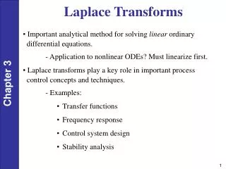
2. Laplace transformation • The Laplace transform is a mathematical technique used for solving linear differential equations (apparent zero order and first order) and hence is applicable to the solution of many equations used for pharmacokinetic analysis.

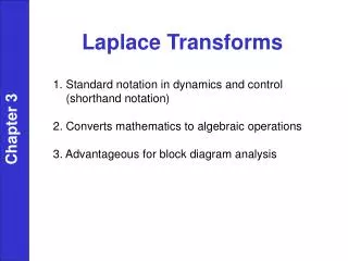
3. Laplace transformation procedure • Write the differential equation • Take the Laplace transform of each differential equation using a few transforms (using table in the next slide) • Use some algebra to solve for the Laplace of the system component of interest • Finally the 'anti'-Laplace for the component is determined from tables

4. Important Laplace transformation (used in step 2) where s is the laplace operator, is the laplace integral , and X0 is the amount at time zero

5. Anti-laplce table (used in step 4)

6. Anti-laplce table continued (used in step 4)

7. Laplace transformation: example • The differential equation that describes the change in blood concentration of drug X is: Derive the equation that describe the amount of drug X??

8. Laplace transformation: example • Write the differential equation: • Take the Laplace transform of each differential equation:

9. Laplace transformation: example • Use some algebra to solve for the Laplace of the system component of interest • Finally the 'anti'-Laplace for the component is determined from tables

10. Laplace transformation: example • The derived equation represent the equation for IV bolus one compartment

11. Continuous intravenous infusion(one-compartment model) Dr Mohammad Issa

12. The drug is administered at a selected or calculated constant rate (K0) (i.e. dX/dt), the units of this input rate will be those of mass per unit time (e.g.mg/hr). The constant rate can be calculated from the concentration of drug solution and the flow rate of this solution, For example, the concentration of drug solution is 1% (w/v) and this solution is being infused at the constant rate of 10mL/hr (solution flow rate). So 10mL of solution will contain 0.1 g (100 mg) drug. The infusion rate (K0) equals to the solution flow rate multiplied by the concentration In this example, the infusion rate will be 10mL/hr multiplied by 100 mg/10 mL, or 100mg/hr. The elimination of drug from the body follows a first Theory of intravenous infusion

13. IV infusion During infusion Post infusion

14. IV infusion: during infusion where K0 is the infusion rate, K is the elimination rate constant, and Vd is the volume of distribution

15. Steady state ≈ steady state concentration (Css)

16. Steady state • At steady state the input rate (infusion rate) is equal to the elimination rate. • This characteristic of steady state is valid for all drugs regardless to the pharmacokinetic behavior or the route of administration.

17. Fraction achieved of steady state concentration (Fss) since , previous equation can be represented as:

18. Fraction achieved of steady state concentration (Fss) or

19. Time needed to achieve steady state time needed to get to a certain fraction of steady state depends on the half life of the drug (not the infusion rate)

20. Example • What is the minimum number of half lives needed to achieve at least 95% of steady state? • At least 5 half lives (not 4) are needed to get to 95% of steady state

21. Example • A drug with an elimination half life of 10 hrs. Assuming that it follows a one compartment pharmacokinetics, fill the following table:

22. Example

23. Example

24. IV infusion + Loading IV bolus • During constant rate IV administration, the drug accumulates until steady state is achieved after five to seven half-lives • This can constitute a problem when immediate drug effect is required and immediate achievement of therapeutic drug concentrations is necessary such as in emergency situations • In this ease, administration of a loading dose will be necessary. The loading dose is an IV holus dose administered at the time of starting the IV infusion to achieve faster approach to steady state. So administration of an IV loading dose and starting the constant rate IV infusion simultaneously can rapidly produce therapeutic drug concentration. The loading dose is chosen to produce Plasma concentration similar or close to the desired plasma concentration that will be achieved by the IV infusion at steady state

25. IV infusion + Loading IV bolus

26. IV infusion + Loading IV bolus • To achieve a target steady state conc (Css) the following equations can be used: • For the infusion rate: • For the loading dose:

27. IV infusion + Loading IV bolus • The conc. resulting from both the bolus and the infusion can be described as: Ctotal =Cinfusion + Cbolus

28. IV infusion + Loading IV bolus: Example • Derive the equation that describe plasma concentration of a drug with one compartment PK resulting from the administration of an IV infusion (K0= Css∙Cl ) and a loading bolus (LD= Css∙Vd) that was given at the start of the infusion

29. IV infusion + Loading IV bolus: Example Ctotal =Cinfusion + Cbolus • Cinfusion: • Cbolus:

30. IV infusion + Loading IV bolus: Example Ctotal =Cinfusion + Cbolus

31. Case A Infusion alone (K0= Css∙Cl) Case B Infusion (K0= Css∙Cl) loading bolus (LD= Css∙Vd) Concentration Concentration Half-lives Half-lives Case C Infusion (K0= Css∙Cl) loading bolus (LD > Css∙Vd) Case D Infusion (K0= Css∙Cl) loading bolus (LD< Css∙Vd) Concentration Concentration Half-lives Half-lives Scenarios with different LD

32. Changing Infusion Rates Increasing the infusion rate results in a new steady state conc. 5-7 half-lives are needed to get to the new steady state conc Concentration Half-lives 5-7 half-lives are needed to get to steady state Decreasing the infusion rate results in a new steady state conc. 5-7 half-lives are needed to get to the new steady state conc

33. Changing Infusion Rates • The rate of infusion of a drug is sometimes changed during therapy because of excessive toxicity or an inadequate therapeutic response. If the object of the change is to produce a new plateau, then the time to go from one plateau to another—whether higher or lower—depends solely on the half-life of the drug.

34. Post infusion phase During infusion Post infusion C* (Concentration at the end of the infusion)

35. Post infusion phase data • Half-life and elimination rate constant calculation • Volume of distribution estimation

36. Elimination rate constant calculation using post infusion data • K can be estimated using post infusion data by: • Plotting log(Conc) vs. time • From the slope estimate K:

37. Volume of distribution calculation using post infusion data • If you reached steady state conc (C* = CSS): • where k is estimated as described in the previous slide

38. Volume of distribution calculation using post infusion data • If you did not reached steady state (C* = CSS(1-e-kT)):

39. Example 1 Following a two-hour infusion of 100 mg/hr plasma was collected and analysed for drug concentration. Calculate kel and V.

40. Time is the time after stopping the infusion

41. Example 1 • From the slope, K is estimated to be: • From the intercept, C* is estimated to be:

42. Example 1 • Since we did not get to steady state:

43. Example 2 • Estimate the volume of distribution (22 L), elimination rate constant (0.28 hr-1), half-life (2.5 hr), and clearance (6.2 L/hr) from the data in the following table obtained on infusing a drug at the rate of 50 mg/hr for 16 hours.

44. Example 2

45. Example 2 • Calculating clearance: It appears from the data that the infusion has reached steady state: (CP(t=15) = CP(t=16) = CSS)

46. Example 2 • Calculating elimination rate constant and half life: From the post infusion data, K and t1/2 can be estimated. The concentration in the post infusion phase is described according to: where t1 is the time after stopping the infusion. Plotting log(Cp) vs. t1 results in the following:

47. Example 2

48. Example 2 K=-slope*2.303=0.28 hr-1 Half life = 0.693/K=0.693/0.28= 2.475 hr • Calculating volume of distribution:

49. Example 3 • A drug that displays one compartment characteristics was administered as an IV bolus of 250 mg followed immediately by a constant infusion of 10 mg/hr for the duration of a study. Estimate the values of the volume of distribution (25 L), elimination rate constant (0.1hr-1), half-life (7), and clearance (2.5 L/hr) from the data in the following table

50. Example 3