Imaging Solar Coronal Structure With TRACE
480 likes | 494 Views
Explore the major physics problems of the solar corona, including its temperature, structure, and dynamics, using X-ray observations from the TRACE satellite. Analyze steady outflows, transient loop brightenings, steady heating of hot loops, and flare-like events in active regions.

Imaging Solar Coronal Structure With TRACE
E N D
Presentation Transcript
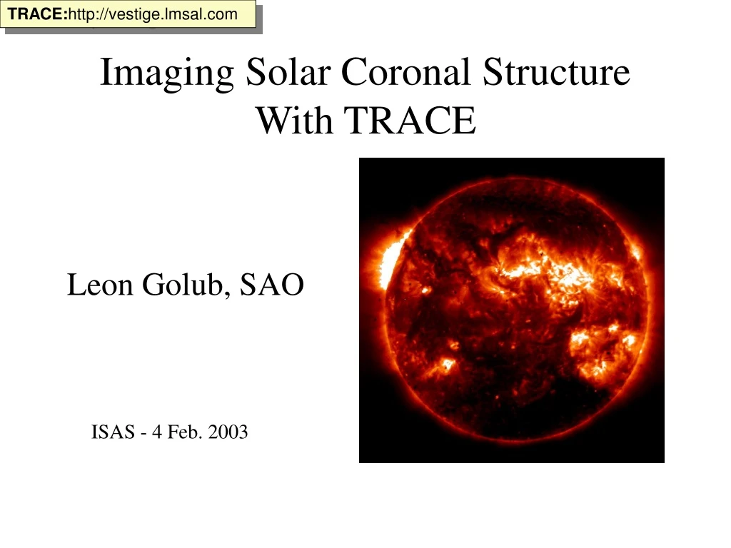
TRACE:http://vestige.lmsal.com Imaging Solar Coronal Structure With TRACE Leon Golub, SAO ISAS - 4 Feb. 2003
http://hea-www.harvard.edu/SSXG/ The SAO Solar-Stellar X-ray Group • Leon Golub • Jay Bookbinder • Ed DeLuca • Mark Weber • Joe Boyd • Paul Hamilton • Dan Seaton • With results from A. Van Ballegooijen, A. Winebarger and H. Warren
The Major Coronal Physics Problems 1. Why is the corona hot? 2. Why is the corona structured? 3. Why is the corona dynamic & unstable? Emergence of B into the atmosphere, and response to B.
Heating & Dynamics in ARs TRACE sees four (or possibly only three) distinct processes in active regions: 1. Steady outflows in long, cool structures. ◄ 2. Transient loop brightenings in emerging flux areas. Also hot & cool material intertwined – May or may not be related to TLBs. 3. Steady heating of hot loops (moss). ◄ 4. Flare-like events at QSLs (or may be cooling events predicted by 3.).
TRACE Active Region Observations are not Consistent With Hydrostatic Model Figure from Aschwanden et al. 2000
Non-HS Loops are ubiquitous courtesy H. Warren
Lenz etal 1999, ApJ, 517, L155. Aschwanden etal 2000, ApJ, 531, 1129. Winebarger etal 2001, ApJ, 553, L81. Schmelz etal 2001, ApJ, 556, 896. Chae etal 2002, ApJ, 567, L159. Testa etal 2002. ApJ, 580, in press. Martens etal 2002, ApJ, 577, L115. Schmelz 2002, ApJ, 578, L161. Aschwanden 2002 ,ApJ, 580, L79. Warren etal 2003, ApJ, submitted. Small gradient in filter ratio, high n. Multithread model (a la Peres etal 1994, ApJ 422, 412), footpoint heating. Flows and transient events in non-hydrostatic loops. DEM spread → const. filter ratio. More passbands may help. Large range in thread T for some loops. Full DEM need at each point. Grad T along loops w/flat filter ratio Contra Martens. Repeated heating episodes. Partial Listing of Recent Papers About Non-Hydrostatic Loops
What Needs to be Explained? • 1. 195A/173A ratio is flat. • 2. Emission extends too high for hydrostatic loop (this is debated, though). • 3. Loop density is high by an order of magnitude. • 4. Apparent flows (and some Doppler shifts measured).
Winebarger etal ApJL (2001) Static vs. Flow Model
Footpoints in Transient Heating 1. Initial energy release along current sheet (“spotty”) 2. Footpooint brightening. 3. Evaporation, then post-flare loops.
Hot Material in the Corona Mg XII Ly-α superposed on Fe X (log T = 6.9 and 6.0) Consistent with RHESSI detection of non-thermal electrons in “quiescent” active regions.
Warren & Warshall,ApJL (2001) March 17, 2000 M1.1: TRACE 1600 Å Movie
TRACE Footpoint vs. BATSE HXR →HESSI!
The Solar-B Instrument Complement 1. Solar Optical Telescope with Focal Plane Package (FPP) - 0.5m Cassegrain, 480-650nm - VMG, Spectrograph - FOV 164X164 arcsec 2. EUV Imaging Spectrograph (EIS) - Stigmatic, 180-204, 240-290Å - FOV 6.0X8.5 arcmin 3. X-ray Telescope (XRT) - 2-60Å - 1 arcsec pixel - FOV 34X34 arcmin
XRT vs. SXT Comparison 1. Higher spatial resolution: 1.0” vs. 2.5” 2. Higher data rate: 512kB continuous. 3. Ten focal plane analysis filters. 4. Extended low-T and high-T response. 5. FIFO buffer for flare-mode obs.
Science Themes • Plasma Dynamics • Thermal Structure and Stability • The Onset of Large Scale Instabilities • Non-Solar Objects
Plasma Dynamics • Reconnection • loop-loop interaction • flux emergence • nano-flares • AR jets • macro-spicular jets • filament eruption
Plasma Dynamics • Waves • origin of high speed wind • tube waves • coronal seismology Figures from Nakariakov et al. (1999): decaying loop oscillations seen in TRACE can be used to estimate the coronal dissipation coefficient. Re ~ 6 x 10⁵ or Rm ~ 3 x 10⁵ , about 8 orders of magnitude less than classical values.
Thermal Structure/Stability • Physical Properties • Te, ne, EM • energetics • variability timescales • Multithermal Structure • steady loops • filaments
Onset of Large Scale Instabilities • Emerging Flux Region • twisting/untwisting • reconnection • delta Spots • current sheets • topology changes • Active Filaments • Te, ne • local heating
Non-Solar Objects • Jupiter • S VII @ 198 • Nearby RS Cvns • Galaxy Cluster Halos • Comets • Any EUVE source within 1 deg of Sun
Science Drivers I: Spatial Scales 105 km 103 km 101 - 103 km <10 km <10 km • “Global” MHD Scales • Active Regions; • granulation scales • Transverse scales - dT, dn - dB^ and j • Reconnection sites • location • size • dynamics RAM discovery space
Science Drivers II: Time Scales • ~10 sec • ~100 sec • ~1 - 10 sec • ~10 - 100 sec • 1 - 100 sec • minutes - months • Loop Alfven time • Sound speed vs. loop length • Ion formation times • Plasma instability times • Transverse motions • Surface B evolution times