Download
1 / 22
220 likes | 433 Views
Empirical Testing of Solar Coronal and Solar Wind Models. Lauren Woolsey University of Maryland - College Park (2011) Mentor: Dr. Leonard Strachan. Introduction. What is the Solar Wind? * Outflow of particles discovered theoretically in 1958 and experimentally in 1962.

E N D
Empirical Testing of Solar Coronal and Solar Wind Models • Lauren Woolsey • University of Maryland - College Park (2011) • Mentor: Dr. Leonard Strachan
Introduction What is the Solar Wind? * Outflow of particles discovered theoretically in 1958 and experimentally in 1962. * Two regimes of solar wind Coronal Holes and Streamer belts? * Coronal Holes have open field lines, source of fast solar wind. * Non-thermal heating may be significant factor in wind generation. Models can help determine mechanisms. Research Goal: * Use the thermodynamic MAS model output to compare synthesized emission line profiles to those from UVCS observations. * In this way, we hope to verify if the processes used in the model correctly describe the corona and solar wind. Image: http://www.mreclipse.com/SEphoto/ TSE1991/image/TSE91-4cmp1w.JPG
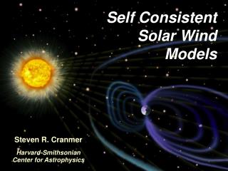
Introduction (continued) Experimental Approach * Two main types of science activity: theory and experiment * By comparing models with observations, we can: a) help to constrain parameters used in theoretical models b) propose new observations to verify model predictions * Forward modeling allows for comparison of model with observation. Model parameters are converted into observables. * Role of UV spectroscopic observations: Line-of-sight profiles provide estimates for plasma parameters such as densities, temperatures, and outflow speeds, which allow energetics to be constrained. Self-consistent coronal/solar wind models * The model only takes inputs at the base of the corona * A change in the magnetic field will alter the plasma parameters, which then change the field.
SOHO: Our Data Source * UVCS (Ultraviolet Coronagraph Spectrometer) ~Instrument on SOlar and Heliospheric Observatory ~Spectral lines include H Lyα and O VI 1032 & 1037 Å LEFT: https://www.cfa.harvard.edu/~scranmer/SSU/soho_inlab_large.gif RIGHT: http://celebrating200years.noaa.gov/breakthroughs/coronagraph/soho_650.jpg
SOHO: UVCS Synoptic Data * Exposures at different heights for Lyα and OVI channels • Slit has 360 rows of 7” pixels, which provides 42’ length. • For Lyα (1216 Å) Observations: • Spectral Resolution is 0.23 Å • Spatial Resolution range is • 12” x 15” – 24” x 24” • Hard stop at 270° • At low heights, synoptic fields of view overlap for full coverage; higher, there are gaps in the data. • For model comparisons, UVCS data were interpolated to make a denser grid.
SOHO: Data Analysis * Data Analysis Software (DAS) v.40 calibrates raw UVCS data into physical units * Gaussian fits to the data determine total intensities and 1/e widths DATA MAP At left, Quick Look image from DAS40. At Right: H Ly α Below: O VI lines
MAS: Modeling the Corona * The model tested is an MHD model of the Corona named Magnetohydrodynamics Around a Sphere (MAS). * Developers: J. Linker, Z. Mikić, R. Lionello, P. Riley, N. Arge, and D. Odstrcil * One of the more complex solar wind models available, but it is only a one-fluid model (not physical for a plasma) * Solves MHD equations for steady state or dynamical solutions Image: http://www.predsci.com/corona/ jul10eclipse/fl_ec1012_007_terrestrial.jpg
n0 = 2 x 1012 cm-3 Relaxation to Steady State T0 = 20,000 K From the B-field Temperature NSO at Kitt Peak SOLAR WIND PARAMETERS: 1 – 20 solar radii and radiation loss term Hch= Hexp+ HQS+ HAR Q(t) from Athay (1986)
MAS: 3D Grid to 1D Line * For each solar rotation, the model returns 3D arrays of data for V (shown), Ne, Te, and B, which we plot at different radii, latitudes, and longitudes. * UVCS integrates along a specified line of sight (LOS), model must match. * Defining a LOS: Polar Angle, Height, Endpoints * Once the model data is defined along a line of sight, spectral profiles produced with the model plasma parameters can be compared with the UVCS observed profiles.
Compare: CORPRO * CORPRO computes a LOS-integrated spectral profile I(λ) At each LOS point, calculate emissivity (ne, v, Te, Tp): The total intensity is a sum of these emissivities 1/e width is fitted directly from integrated profile * Profiles can be plotted to get visual comparison * Model provides a single value for T, we must determine its components
Case 1: Assume Tmodel = Te * Solve Tp by matching Imodel = Iobs * Electron temperature controls ionization fraction N(P) term in total intensity * Proton Temperature is a “kinetic temperature.” It controls the 1/e width. However, Tp can also affect total intensity through Doppler dimming. * Tp is determined by adjusting the parameter until the modeled intensity matches observed intensity (within data uncertainty) * 1σ observational error bars may be smaller than symbols. No model error was provided.
Case 1: Sample Lyα profiles Streamer at 2.5 Rsun Coronal Hole at 2.5 Rsun * Tp is reasonable in a streamer * Tp is unphysical in coronal hole and provides a poor match to the observations. *Need a better way to include T in the CORPRO model for a coronal hole.
Case 2: Assume Tmodel = Tavg * Goal is to improve the coronal hole (CH) comparison * Include non-thermal term in proton temperature: Tp is a kinetic temperature: ½mv2 = kT Tp = (m/2k)(vth2 + vnon2) * Most likely source of non-thermal velocity is from Alfvén waves, which are included in MAS model Table: Best α value where Imod = Iobs Tavg = ½(Te + Tp) Te = α Tavg Tp = (2 – α) Tavg
Case 2: Results for CH * For a fixed α, vnt can be determined using the model for vnt vs. r at right and B, n, and v parameters from MAS model to match line widths. * Non-thermal velocities: 89.8 km/s at 1.7 Rsun 90.3 km/s at 2.0 Rsun Landi & Cranmer (2009) Left: Coronal Hole @ 1.7 Rsun; Right: @ 2.0 Rsun
Summary of Results * STREAMER ★ Generally, the equatorial region (the slow-wind regime) is well-described by the MAS model when using case 1 (Tmod = Te). * CORONAL HOLE ★ Te is increasing at 2 Rsun with no sign of a turnover below 2.25 Rsun. ★ Non-thermal velocities are roughly 90 km/s for protons (most UVCS studies focus on OVI ions) ★ With the set of values determined for α and vnt there is excellent agreement between MAS model and observations. * While agreement is good, it is not unique.
Future Work * Examine the MAS model and other MHD models for other periods in the solar cycle * Incorporate the data from O VI to add further constraints to the model parameters * Study an active region in the corona to see how shaped empirical heating function compares to observations Recommendations * MAS model should incorporate separate Te and Tp parameters (two-fluid physics) in order to be more physically accurate, or provide a better definition of which single temperature is calculated.
References Akinari, N. (2007). Broadening of resonantly scattered ultraviolet emission lines by coronal hole outflows. ApJ, 660: 1660-1673. Cranmer et al. (1999). An empirical model of a polar coronal hole at solar minimum. ApJ, 511: 481. Jacques, S.A. (1977). Momentum and energy transport by waves in the solar atmosphere and solar wind. ApJ, 215: 942-951. Kohl et al. (1995). The Ultraviolet Coronagraph Spectrometer for the Solar and Heliospheric Observatory. Solar Physics, 162(1-2): 313-356. Landi, E. and Cranmer, S.R. (2009). Ion temperatures in the low solar corona: Polar coronal holes at solar minimum. ApJ, 691: 794-805. Lionello, R., J.A. Linker, and Z. Mikić (2009). Multispectral emission of the Sun during the first whole Sun month: Magnetohydrodynamics simulations. ApJ, 690: 902-912. Ong et al. (1997). Self-consistent and time-dependent solar wind models. ApJ, 474: L143-L145. Withbroe, G.L., J.L. Kohl, and H. Weiser (1982). Probing the solar wind acceleration region using spectroscopic techniques. Space Science Reviews, 33: 17-52. THANK YOU!
UVCS Instrument Parameters * Ly-α channel Ruling frequency: 2400 l/mm Angle of incidence α: 12.85° Angle of diffraction β: 3.98° Main radius of curvature: 750 mm Minor radius of curvature: 729.5 mm Reciprocal Dispersion: 5.54 Å/mm (1st order) Spectral Bandwidth of pixel: 0.14 Å (1st order) Spatial width of pixel: 0.025 mm Image: http://www.chrismadden.co.uk/moon/micro.html
Carrington Rotations * Model takes a base synoptic magnetogram from a full Carrington Rotation (e.g. from NSO at Kitt Peak) * One CR represents a full solar rotation from a point when 0° longitude faces Earth to the next. DATE LONGITUDE Image from http://people.hao.ucar.edu/sgibson/wholesun/DATA/AGU_CORONAL/wsm_195_merid_150_lab.gif
Parameters from Line Width If absence of non-thermal velocities (e.g. Alfvén waves): V1/e = c*Δλ1/e/λ0 V1/e = sqrt(2kT/m) T = (m/2k)*V1/e2 = (mc2/2kλ02)*Δλ1/e2 Lyα 1216 Å from H (m = proton mass) V1/e = 246.6*Δλ1/e V1/e = sqrt( T/60.5 ) T = ( 3.68 x 10⁶ ) Δλ1/e2 1032 Å from OVI (m = 16*proton mass) V1/e = 291*Δλ1/e V1/e = sqrt( T/965 ) T = ( 81.7 x 10⁶ ) Δλ1/e2
MAS Model UVCS Data CORPRO DAS v40 Data Map “Modeled” { Itot, Δλ1/e } {n,v,T,B} Goal is to search for consistency between the MAS model and the UVCS Data by using Forward Modeling. “Observed” { Itot, Δλ1/e } { I(rows,col) } { I(λ) }