Using GIS to Find Suitable Locations for Solar Power Plants Submitted By: Scott Peterson

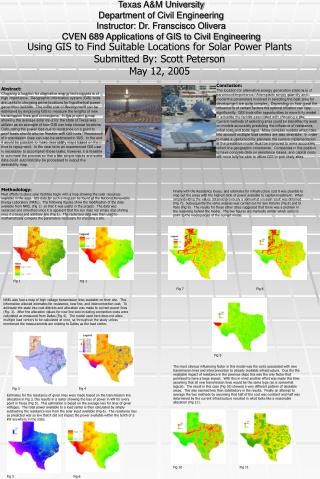
1. Texas A&M UniversityDepartment of Civil EngineeringInstructor: Dr. Franscisco OliveraCVEN 689 Applications of GIS to Civil Engineering Using GIS to Find Suitable Locations for Solar Power Plants Submitted By: Scott Peterson May 12, 2005 Conclusion: The location for alternative energy generation stations is of paramount importance. Attempts to simply quantify and model the parameters involved in selecting the best area for development are quite complex. Depending on how great the influence is of certain factors the optimal location can vary significantly. GIS tools offer opportunities to more fully model in advance the factors associated with choosing a site. Current methods of selecting sites could be benefited by work on models accurately predicting the influence of resistance, initial cost, and solar input. More complex models which take into account multiple load centers are also desirable. In order to make a useful tool for planners the current implementation of the predictive model must be improved to more accurately reflect the geographic constraints. Companies in the position to have concrete data on resistance losses, and capital costs will more fully be able to utilize GIS to pick likely sites. Abstract: Choosing a location for alternative energy technologies is of high importance. Geographic information system (GIS) tools are useful in choosing prime locations for hypothetical power generation facilities. The initial cost of development can be estimated by employing GIS to measure the lengths of new transmission lines and connections. In this project a map showing the average solar input for the state of Texas was utilized as an example of how GIS can help choose locations. Calculating the power loss due to resistance on a point to point basis should also be feasible with GIS tools. Resistance of transmission lines can also be estimated in GIS. In the end it would be possible to make desirability maps based on the time to repayment. In the near term an experienced GIS user is necessary to accomplish these tasks; however, it is feasible to automate the process so that a few simple inputs and some data could automatically be processed to output the desirability map. Methodology: Most efforts to place solar facilities begin with a map showing the solar resources available in the area. GIS data for such a map can be found at the National Renewable Energy Laboratory (NREL). The following figures show the modification of the data available from NREL (Fig 1) so that it was useful in the project. The data was rasterized and smoothed since it is apparent that the sun does not simply stop shining once it crosses and arbitrary line (Fig 2). The rasterized data was then used to mathematically compute the parameters necessary for choosing a site. Finally with the Resistance losses, and estimates for infrastructure cost it was possible to map out the areas with the highest ratio of power available to capital investment. When simply dividing the values obtained previously a somewhat unusual result was obtained (Fig 7). Subsequently the same analysis was carried out for San Antonio (Fig 8) and El Paso (Fig 9). The results for these other cities suggested that there was a problem in the reasoning behind the model. The two figures are markedly similar which sems to point to the inadequacies of the current model. Fig 1 Fig 2 Fig 7 Fig 8 NREL also had a map of high voltage transmission lines available on their site. This information allowed estimates for resistance, new line, and interconnection cost. To delineate the state into cost districts and allocation was made to current power lines (Fig. 3). After the allocation values for new line cost including connection costs were calculated as measured from Dallas (Fig 4). The model used here does not allow multiple load centers to be calculated at once, so throughout the study unless mentioned the measurements are relating to Dallas as the load center. Fig 9 The most obvious influencing factor in this model was the costs associated with new transmission lines and interconnection to already available infrastructure. Due the the negligible impact of resistance in the previous steps this was the only factor that promised to have a large impact. With this in mind another effort was made this time assuming that all new transmission lines would be the same type (as is somewhat logical). The result in this case (Fig 10) showed a very different pattern of desirable areas. This also seemed less than satisfactory in the results. Finally an attempt to average the two methods by assuming that half of the cost was constant and half was determined by the current infrastructure resulted in what looks like a reasonable allocation (Fig 11). Fig 3 Fig 4 Estimates for the resistance of given lines were made based on the transmission line allocation in Fig 3, this results in a raster showing the loss of power in kW for every point in Texas (Fig 5). This estimation is based on the average loss for lines of given voltages. The total power available to a load center is then calculated by simply subtracting the resistance loss from the solar input available (Fig 6). The resistance loss as predicted was so low that it did not impact the power available within the tenth of a kW anywhere in the state. Fig 10 Fig 11 Fig 5 Fig 6