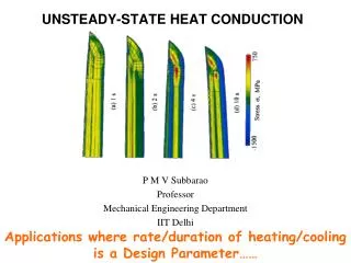
Two Dimensional Steady State Heat Conduction
Two Dimensional Steady State Heat Conduction. P M V Subbarao Associate Professor Mechanical Engineering Department IIT Delhi. It is just not a modeling but also feeling the truth as it is…. l 2 < 0 or l 2 > 0 Solution. OR. q = C. Any constant can be expressed as

Two Dimensional Steady State Heat Conduction
E N D
Presentation Transcript
Two Dimensional Steady State Heat Conduction P M V Subbarao Associate Professor Mechanical Engineering Department IIT Delhi It is just not a modeling but also feeling the truth as it is…
l2 < 0 or l2 > 0 Solution OR q = C Any constant can be expressed as A series of sin and cosine functions. H q = 0 q = 0 y l2 > 0 is a possible solution ! 0 W x q = 0
Solution domain is a superset of geometric domain !!! Recognizing that
where the constants have been combined and represented by Cn Using the final boundary condition:
Construction of a Fourier series expansion of the boundary values is facilitated by rewriting previous equation as: where
And hence Substitutingf(x) = T2 - T1into above equation gives:
Isotherms and heat flow lines are Orthogonal to each other!
q = Cx H q = 0 q = 0 y Linearly Varying Temperature B.C. 0 W x
Sinusoidal Temperature B.C. q = Cx H q = 0 q = 0 y 0 W x
Principle of Superposition P M V Subbarao Associate Professor Mechanical Engineering Department IIT Delhi It is just not a modeling but also feeling the truth as it is…
For the statement of above case, consider a new boundary condition as shown in the figure. Determine steady-state temperature distribution.
If m is a total number of the heat flow lanes, then the total heat flow is: Where S is called Conduction Shape Factor.
Conduction shape factor Heat flow between two surfaces, any other surfaces being adiabatic, can be expressed by where S is the conduction shape factor • No internal heat generation • Constant thermal conductivity • The surfaces are isothermal Conduction shape factors can be found analytically shapes
Thermal Model for Microarchitecture Studies • Chips today are typically packaged with the die placed against a spreader plate, often made of aluminum, copper, or some other highly conductive material. • The spread place is in turn placed against a heat sink of aluminum or copper that is cooled by a fan. • This is the configuration modeled by HotSpot. • A typical example is shown in Figure. • Low-power/low-cost chips often omit the heat spreader and sometimes even the heat sink;
Thermal Circuit of A Chip • The equivalent thermal circuit is designed to have a direct and intuitive correspondence to the physical structure of a chip and its thermal package. • The RC model therefore consists of three vertical, conductive layers for the die, heat spreader, and heat sink, and a fourth vertical, convective layer for the sink-to-air interface.
Multi-dimensional Conduction in Die The die layer is divided into blocks that correspond to the microarchitectural blocks of interest and their floorplan.
For the die, the Resistance model consists of a vertical model and a lateral model. • The vertical model captures heat flow from one layer to the next, moving from the die through the package and eventually into the air. • Rv2in Figure accounts for heat flow from Block 2 into the heat spreader. • The lateral model captures heat diffusion between adjacent blocks within a layer, and from the edge of one layer into the periphery of the next area. • R1 accounts for heat spread from the edge of Block 1 into the spreader, while R2 accounts for heat spread from the edge of Block 1 into the rest of the chip. • The power dissipated in each unit of the die is modeled as a current source at the node in the center of that block.
Thermal Description of A chip • The Heat generated at the junction spreads throughout the chip. • And is also conducted across the thickness of the chip. • The spread of heat from the junction to the body is Three dimensional in nature. • It can be approximated as One dimensional by defining a Shape factor S. • If Characteristic dimension of heat dissipation isd