Download
1 / 40
640 likes | 1.19k Views
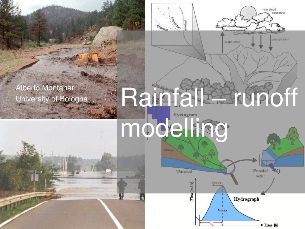
Rainfall – runoff modelling. Alberto Montanari University of Bologna. What hydrology should do for water resources management?. Hydrology should provide the required information to water resources managers: Water Resources Availability. Water Quality.

E N D
Rainfall – runoff modelling Alberto Montanari University of Bologna
What hydrology should do for water resources management? Hydrology should provide the required information to water resources managers: • Water Resources Availability. • Water Quality. • Technical strategies for managing water resources. Issue 1 is compelling. Lack of historical information and problems related to river discharge measurement make estimation of water resources availability a relevant technical problem.
Hydrologycal cycle Figure 7.1.1 (p. 192)Hydrologic cycle with global annual average water balance given in units relative to a value of 100 for the rate of precipitation on land (from Chow et al. 1988)).
The Hydrologic Cycle as a FlowchartProcesses understanding We want to estimate the amount of water moved by the different processes! Figure 7.1.3 (p. 193)Block-diagram representation of the global hydrologic system from Chow et al. (1988)).
How hydrological processes can be modelled? • Hydrologicalmodelstrytoschematise the dynamicsof water flow within the water cycle. Therefore,they deal with transfer of mass whichmay take place in differentphases (solid, liquid, gas). Such mass transfersoccurthroughexchangesofenergy. • Conservationof mass and energy are alwaysverified in fluidmechanics, aswellas Newton’s laws: • Every object in a state of uniform motion tends to remain in that state of motion unless an external force is applied to it. • The relationship between an object's mass m, its acceleration a, and the applied force F is F = ma. Acceleration and force are vectors. • For every action there is an equal and opposite reaction.
How hydrological processes can be modelled? • Therefore, ifonewishestoreproducewithmathematicalrelationships the dynamicsofhydrologicalprocesses, the continuityequation and energy and momentumconservation can beapplied. • Hydrologicalprocesses are typicallyheterogeneous and highlyvarying in time and therefore the abovebalanceequationare oftenexpressed in differentialform, byreferringtoelementaryspaceunits or a single particleoffluid. We can assume heterogeneity and stationaritywhenreferringtoelementaryareas and infinitesimaltimesteps.
Control volume and Reynolds transport theorem • Balanceequationsneedtobeappliedbyreferringto a control volume. • In fluid mechanics and thermodynamics, a control volume is a mathematical abstraction employed in the process of creating mathematical models of physical processes. In an inertial frame of reference, it is a volume fixed in space or moving with constant velocity through which the fluid (gas or liquid) flows. The surface enclosing the control volume is referred to as the control surface. • Balance equations for any extensive property within a control volume can be expressed through Reynolds Transport Theorem: • where B is an extensive property of the fluid (like total mass or momentum of the system), b is its intensive counter part (property per unit mass of fluid),ris the mass density of the fluid, V is control volume, S is its control surface, u is the flow velocity vector and n is the outgoing unit normal vector.
The Watershed Figure 7.1.4 (p. 194)Schematic diagram of a drainage basin. The high terrain on the perimeter is the drainage divide (from Marsh (1987)).
Watershed Delineation We derive watershed divides from paper or digital maps. We start from a point on the river and move perpendicular to the contour lines to the top of the contours (the divide).
Runoff Watershed Rainfall-Runoff Model Rainfall Runoff Rainfall-Runoff Modeling Rainfall
Rainfall-Runoff Modeling Hyetograph Hydrograph
Rainfall-Runoff Modeling • Input: • Simulation behaviours and requirements (time step, type of model, computational requirements….); • Catchment behaviours (soil type and use, catchment area, catchment elevation….); • River network behaviours (geometry of the cross river sections, roughness of the river bed, slope of the river bed….); • Meteorological input (rainfall, snowfall, temperature, wind speed and direction…..). • Output: • River flow (possibly in more than one cross river section…..); • Evapotranspiration, water storage….. • Design variables.
Rainfall-Runoff Modeling • Modelstructure: • Lumped vs spatially distributed; • Black box vs conceptual vs physically-based; • Event based versus continuous simulation; • Simulation models vs forecasting models. • Parameters: • A parameter is a constant or variable term in a function that determines the specific form of the function but not its general nature, as a in f (x) = ax, where a determines only the slope of the line described by f(x). • Parameters might be present in fully physically-based equations (physical properties can be considered as parameters) but usually the term parameter is reserved for quantities that are not physically measurable and compensate for approximations in physical equations. • Calibration and validation.
Modeling Considerations • Development of a rainfall-runoff model depends on (1) Time scale (2) Basin scale • Small basin operate a less significant filtering effect on rainfall. • Linear models are not appropriate for short time scales and small spatial scales. • Constant and spatially uniform rainfall typically induces a S-shaped hydrograph in the long time. • It is important to gain a full comprehension of the rainfall-runoff transformation on a perceptional basis. Go out and look around, especially during floods!
Rational Formula • First proposed by Kuichling in 1889 • Qp = C i A where Qp= peak discharge (m3/s); i = rainfall intensity (m/s) A = drainage area (m2) C = runoff coefficient ( - ) depending on water losses • Note: i = average intensity of rainfall corresponding to the duration of time-to-concentration.
Time-of-Concentration • Definition: the time needed for water to flow from the most remote point in a watershed to the watershed outlet. It is very difficult to measure. Runoff coefficient • Again, it is very difficult to measure.
Time-Area Method • Can be considered as an extension of the rational method in which rainfall intensity in not uniform over the storm duration
Linear Reservoir Method Accordingly to this model, the catchment is assimilated to a reservoir and the river discharge at the outlet is assumed to be given by the outflow from a bottom discharge. The discharge is assumed to be related to the stored volume by a linear relationship: which can be considered an empirical expression of an energy balance equation (Torricelli’s law).
Linear Reservoir Method We can also impose the continuity equation to the reservoir: which can be considered an empirical expression of an energy balance equation (Torricelli’s law). By combining one obtains:
Linear Reservoir Method By multiplying both sides by et/k one obtains: which can be written as: By integrating between 0 and t one obtains:
Linear Reservoir Method By imposing q(0) = Q0 one obtains: + Q0 e-t/k • Please note: • River discharge is linearly related to the river cross section area; • assuming a linear relationship between river discharge and water stored in the catchment implies a linear relationship between cross section area and water volume stored in the catchment. • This means that the virtual water level shift is uniformly distributed over the catchment (synchronous functioning)
Generalisation of linear methods Linear reservoir (by neglecting Q0): Time-area method: T
Generalisation of linear methods By generalising: where h(t) is called the Instantaneous Unit Hydrograph (IUH). It is the response of the catchment to an (instantaneous) impulse of rainfall of unit volume. Note: for linear systems the principle of superposition of the effects applies. In general, it is not a suitable assumption (but depends on catchments size and time scale). Many different IUHs are proposed by the scientific literature.
Variable source area models Actually, in a river basin the water storage capacity is spatially varying. Figure 2 from Moore, R. J.: The PDM rainfall-runoff model, Hydrol. Earth Syst. Sci., 11, 483-499, doi:10.5194/hess-11-483-2007, 2007
Hymod model Water storagecapacity
Hymod model Assumption: evapotranspiration is null and cumulated rainfall from the beginning of the event is indicated as P(t) W(t) is the volume of water stored in the catchment per unit catchment area
Hymod model se C* is now the storage in the unsaturated part of the catchment
Hymod model EP(t) is potential evapotranspiration E(t) is actual evapotranspiration
Hymod model After subtracting evapotranspiration, at each time step, C*(t) is recomputed through the relationship: Note again that C*(t) is the water depth that is stored in the part of the catchment that is not saturated.
Hymod model The runoffisdivided in twocomponentsthrough a parameter a. The twocomponents are routedthrough a linearreservoir (slow component) and a cascadeofthreereservoirwith the same K value (fast component). Then, the modelcounts a total of 5 parameters.