Download

1 / 17
170 likes | 364 Views
HDR Image Construction from Multi-exposed Stereo LDR Images. Ning Sun, Hassan Mansour, Rabab Ward Proceedings of 2010 IEEE 17th International Conference on Image Processing September 26-29, 2010, Hong Kong. Andy { andrey.korea@gmail.com }. Algorithm description.

E N D
HDR Image Construction from Multi-exposed Stereo LDR Images Ning Sun, Hassan Mansour, Rabab Ward Proceedings of 2010 IEEE 17th International Conference on Image Processing September 26-29, 2010, Hong Kong Andy {andrey.korea@gmail.com}
Algorithm description Two LDR images with different exposures Camera response function Radiance maps of LDR images Refined disparity map HDR image Initial disparity map Main concept: 1. Multi-exposed stereo images are captured using identicalcameras placed adjacent to each other on a horizontal line. 2. Stereo matching is then used to find a disparity map thatmatches each pixel in one image to the corresponding pixelin another image. 3. A subset of the matched pixels is used to generate the cameraresponse function which in turn is used to generate the sceneradiance map for each view with an expanded dynamic range. 4. The disparity map is refined by performing a second stereomatching stage using the radiance maps
Imaging models Left image Right image Correction factor Left image Right image Scene radiance Exposure ration between images Exposure ration between images Scene radiance Imaging models are used to determine the scene radiance from the measured pixel data Gamma-correction model Polynomial camera response
Computing the disparity map Best disparity map Set of feasible disparities Dissimilarity term Smoothing term Used for initial disparity estimation Pixel dissimilarity Disparity smoothness
Pixel dissimilarity Spatial smoothing Intensity smoothing I’ - intensity in log space defined as: - Search window centered on p - Bilateral weight - displacement
Disparity smoothness Initial disparity and camera response 1. Minimize using graph cut algorithm 2. Compute polynomial coefficients for camera response function
Error correction Convert images to radiance space (results should be same for both images) Minimize energy function one more time with different dissimilarity function For valid pixels For erroneous pixels Hamming distance between pixels p and p+fp after applying Census transform
Disparity maps Reference disparity map Initial disparity estimation Final map
Conclusions Disparity map computation algorithm is proposed Proposed method is able to compute disparity between differently exposed images Can deal with saturated regions in the image Can be used for capturing motion scenes with different exposures Disadvantages • - High computational costs • Generated images are slightly blurred • No rotation is considered
Ideal image formation system Camera exposure Radiometric response Camera response function Shutter speed or Image brightness Sensor response Where Reverse camera response function L Irradiance I Response = Gray-level From optics Aperture Angle from ray to optical axis Image radiance Focal length Scene radiance
Response function examples Response functions of a few popular cameras provided by their manufacturers
Graph-cut algorithm 1. Start with an arbitrary labeling f 2. Set success := 0 3. For each label 2 L 3.1. Find f*= argminE(f’) among f’withinoneα-expansion of f 3.2. If E(f*) < E(f), set f := f* and success := 1 4. If success = 1 goto 2 5. Return f
Census transform If (CurrentPixelIntensity<CentrePixelIntensity) boolean bit=0 else boolean bit=1 Input image 3x3 transform 5x5 transform