CCAM simulations for CORDEX South Asia

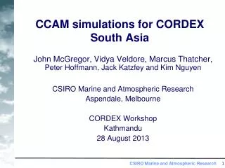
1. CCAM simulations for CORDEX South Asia John McGregor, Vidya Veldore, Marcus Thatcher, Peter Hoffmann, Jack Katzfey and Kim Nguyen CSIRO Marine and Atmospheric Research Aspendale, Melbourne CORDEX Workshop Kathmandu 28 August 2013

2. Introduction to the downscaling approach GCM selection SST bias correction CCAM model features Behaviour of the simulations Outline

3. Downscaling with CCAM Bias correction CCAM (~50 km) GCM (~200 km) CCAM (~14 km) GCM SST/Sea-ice

4. The 50 km run is then downscaled to 10 km by running CCAM with a stretched grid, but applying a digital filter every 6 h to preserve large-scale patterns of the 50 km run A separate 100 km global CCAM run is also used to drive RegCM4.2 at its boundaries for 20 km RCM runs CCAM downscaling methodology • Coupled GCMs have coarse resolution, but also possess Sea Surface Temperature (SST) biases such as the equatorial “cold tongue” • We first run a quasi-uniform 50 km global CCAM run driven by the bias-corrected SSTs Stretched C96 grid with resolution about 14 km over Nepal, showing every 2nd grid point Quasi-uniform C192 CCAM grid with resolution about 50 km, showing every 4th grid point

5. Some previous CCAM downscaling projects Indonesia 14 km Pacific Islands 60 km and 8 km South Africa Australia 20 km – 60 km Tasmania 8 km – 14 km

6. GCM Selection | Peter Hoffmann GCM Selection

7. GCM Selection | Peter Hoffmann GCM Selection Requirements • Good performance in present climate • Simulation of rainfall, air temperature etc. • Reproduce observed trends • Good SSTs • ENSO pattern/frequency • SST distribution • Good spread of climate change signals

8. GCM Selection | Peter Hoffmann GCM Selection Evaluation studies • 24 CMIP5 models • > 20 evaluation studies • 6 publications with rankings + evaluation used within the Vietnam project • Peer-reviewed or submitted

9. GCM Selection | Peter Hoffmann GCM Selection Example: performance in current climate over Indochina Evaluation region Results annual rainfall

10. GCM Selection - Rankings

11. GCM Selection | Peter Hoffmann GCM Selection Final ranking The rankings of the 6 individual studies are averaged to yield a final ranking of the models.

12. GCM SelectionClimate change signal JJA - good spread X X X

13. SST correction

14. Observations • daily optimum interpolation SST & SIC (Reynolds et al., 2007) • 1/4° resolution for 1982-2011 • Method adjust mean adjust variance OBS frequency GCM SST

15. SST bias correction Results: SST BIAS ACCESS1.0 JAN JUL original after correction (K)

16. Results: SST variance ACCESS1.0 (January) Bias & Variance corrected ACCESS1.0 Observed Mean SSTs SST Stdev

17. CCAM is formulated on the conformal-cubic grid Orthogonal Isotropic The conformal-cubic atmospheric model Example of quasi-uniform C48 grid with resolution about 200 km

18. Variable-resolution conformal-cubic grid The C-C grid is moved to locate panel 1 over the region of interest The Schmidt (1975) transformation is applied - it preserves the orthogonality and isotropy of the grid - same primitive equations, but with modified values of map factor C48 grid (with resolution about 20 km over Vietnam

19. atmospheric GCM with variable resolution (using the Schmidt transformation) 2-time level semi-Lagrangian, semi-implicit total-variation-diminishing vertical advection reversible staggering - produces good dispersion properties a posteriori conservation of mass and moisture CCAM dynamics

20. CCAM physics • Cumulus convection:scheme for simulating rainfall processes • Detailed modelling of water vapour, liquid and ice to determine cloud patterns

21. CCAM physics • Cumulus convection:scheme for simulating rainfall processes • Detailed modelling of water vapour, liquid and ice to determine cloud patterns • Parameterization of turbulent boundary layer (near Earth’s surface)

22. CCAM physics • Cumulus convection:scheme for simulating rainfall processes • Detailed modelling of water vapour, liquid and ice to determine cloud patterns • Parameterization of turbulent boundary layer (near Earth’s surface) • Modelling of vegetation and using 6 layers for soil temperatures and moisture • CABLE canopy scheme

23. CCAM physics • Cumulus convection:scheme for simulating rainfall processes • Detailed modelling of water vapour, liquid and ice to determine cloud patterns • Parameterization of turbulent boundary layer (near Earth’s surface) • Modelling of vegetation and using 6 layers for soil temperatures and moisture. 3 layers for snow • CABLE canopy scheme • GFDL parameterization of radiation (incoming from sun, outgoing from surface and the atmosphere)

24. In each convecting grid square there is an upward mass flux within a saturated aggregated plume There is compensating subsidence of environmental air in each grid square As for Arakawa schemes, the formulation is in terms of the dry static energy sk = cpTk + gzk and the moist static energy hk = sk + Lqk Cumulus parameterization

25. Above cloud base subsidence detrainment plume downdraft

26. The Maritime Continent has many islands with land or sea breeze effects, and extra SST variability a) enhance sub-grid cloud-base moisture if diurnal increase of SSTs, or b) enhance sub-grid cloud-base moisture if upwards vertical motion Both (a) and (b) are beneficial over Indonesia, Australia, Vietnam, China – (b) slightly better (b) seems less suitable over India (a) still fine over India Enhancements for Maritime Continent

27. Cloud microphysics scheme (Rotstayn) CCAM carries and advects mixing ratios of water vapour (qg), cloud liquid water (ql) and cloud ice water (qi)

28. Latest GFDL radiation scheme • Provides direct and diffuse components • Interactive cloud distributions are determined by the liquid- and ice-water scheme of Rotstayn (1997). The simulations also include the scheme of Rotstayn and Lohmann (2002) for the direct and indirect effects of sulphate aerosol • Short wave (has H2O, CO2, O3, O2, aerosols, clouds, fewer bands) • Long wave (H2O, CO2, O 3, N 2O, CH4, halocarbons, aerosols, clouds)

29. Tuning/selecting physics options: In CCAM, usually done with 100 km or 200 km AMIP runs, especially paying attention to Australian monsoon, Asian monsoon, Amazon region No special tuning for stretched runs A recent AMIP run 1979-1989 DJF JJA Obs CCAM 100 km

30. CORDEX runs using CCAM • We are performing global runs at 50 km, providing outputs for 4 CORDEX domains: Africa, Australia, SE Asia, S Asia. • RCP 4.5 and 8.5 emissions scenarios • So far have downscaled 6 of the CMIP5 GCMs at 50 km/ L27 resolution (as part of large Vietnam project). Output now available. • Doing more runs, and more at 100 km. • Performing the runs at CSIRO, CSIR_South_Africa, and Queensland_CCCE

31. TRMM JJAS a 100 km a 50 km ERA-I b 50 km – ACCESS Others quite similar a 14 km GPCP JJAS

32. Rainfall change by 2080 (mm/d)JJAS RCP 8.5 CCAM_MPI CCAM_GFDL CCAM_CNRM CCAM_ACCESS

33. % rainfall change by 2080 (mm/d)JJAS RCP 8.5 CCAM_MPI CCAM_GFDL CCAM_CNRM CCAM_ACCESS

34. TRMM-3B43 TRMM GPCP CCAM-100km CCAM-14km CCAM-Coupled 100 & 14 km CCAM-BVC_SST GPCP coupled Over land and sea 50 km runs Convection in 50 km runs included vertical velocity enhancement (b)

35. DJF JJA Obs CCAM 100 km CCAM 14 km over N India stretched

36. 100 km AMIP runs vs CMAP CMAP CCAM CCAM CMAP MAM DJF JJA SON 1979-1989 C96 100 km AMIP run Generally good rainfall. Fresh 50 km CORDEX runs are underway

37. 14 km runs vs Aphrodite Aphrodite CCAM CCAM Aphrodite DJF MAM JJA SON

38. 14 km runs vs IMD obs

39. JJAS present-day rainfall over NEPAL DHM obs CCAM 14 km

40. CCAM coupled model - 14 km over Asia Quite acceptable rainfall

41. 14 km coupled runs – 3 days MSLP, wind vectors, mixed layer depth > 50 m

42. 14 km coupled runs – 3 days SSTs