Download
1 / 19
190 likes | 264 Views
eHeroes. Evolutionary pattern of DEM variations in flare(s). B. Sylwester, J. Sylwester, A. Kępa , T. Mrozek Space Research Centre, PAS, Wrocław , Poland K.J.H. Phillips Natural History Museum, London, UK V.D. Kuznetsov IZMIRAN, Moscow, Russia.

E N D
eHeroes Evolutionary pattern of DEM variations in flare(s) B. Sylwester, J. Sylwester, A. Kępa, T. Mrozek Space Research Centre, PAS, Wrocław, Poland K.J.H. Phillips Natural History Museum, London, UK V.D. Kuznetsov IZMIRAN, Moscow, Russia ApJ submitted, is after the first iteration with the Referee
Average RESIK spectrum spectrum (integratedover26.5 min) for M1.0 flare Well observed flare, 127 individual spectra available, that we summed over 19 time intervals for detailed analysis.
SOL2002-11-14T22:26normalisedlightcurves GOES 0.5 – 4 Å 1 – 8 Å RHESSI 6 – 12 keV 12 – 25 keV 25 – 50 keV Sample spectra for: rise (e), maximum (g) and decay (n) phases 19 timeintervalsselected (a-s)
Spectra evolution: SOL2002-11-14T22:26different colours-individual spectral channels Event Average spectrum Rise phase Maximum phase Decayphase 3 MK 30 MK
RESIK - Braggbentcrystalspectrometer: NRL, MSSL, RAL, IZMIRAN 4 x RESIK aboard the Russian CORONAS-F satellite. It observed solar coronal spectra in four energy bands over ~3.3 Å – 6.1 Å band (~800 spectral bins) Operational in 2002 and first part of 2003 ~ 2 mln spectra available, 6000 reduced to Level2 (60 flares). Data in the public domain http://www.cbk.pan.wroc.pl/experiments/resik/RESIK_Level2/index.html
Selection of spectral bands (for inversion) • 15 bands: • Most of them contain prominent lines of abundant elements • K, Ar, S & Si + cont. • Some preferentially the continuum • For every selected time (interval: a, b..) we take from observations the set of 15 fluxes Fi Si S Si c Ar S K c
The inversion:15measuredfluxes for opticallythinplasma ? DEM always positive, characterizes how much of plasma is present at a particular temperature interval dT (notwithstanding where within FOV) fi(T) CHIANTI (7.0) emission (contribution) function for each predefined spectral band, Tables of Ai * fi(T) have been calculated for a grid of AEL & T (days of calculation using CHIANTI)
Just to show how important is “pre-assumption” of composition on the inversion a Coronal Photospheric Identical sets of input fluxes have been used for a and b. The Withbroe-Sylwester iterative algorithm corresponding to the maximum likelihood Bayesian procedure (Solar Phys., 67, 1980, ) has been used for invertion. The kernel fluxes have been calculated based on the CHIANTI 7.0 code with adopted Photosphericand Coronal plasma composition respectively. Bryans ionization equilibrium has been adopted (ApJ, 691, 2009). 10 000 iterations have been performed in the accelerated scenario and the errors have been estimated from 100 Monte Carlo realizations of DEM calculations. Dramatically different distribution of plasma DEM are unveiled for these different abundance sets
The „AbuOpt” approach • The emission functions for inversion were generated for a number of following abundance pattern scenarios: • For every important element : K, Ar, S & SI the values of kernel Ai * fi(T) were calculated for a set of abundances ranging from • 0.1 to 16 times the accepted „coronal” value of abundance • i.e. 21 different values of abundances for particular element • While changing the abundance of an element „in question”, the other elements’ abundances were being kept to their coronal values when generating the kernel functions. • We „tried” to fit (make inversion) of the observed fluxes for all calculated abundance patterns (~80) using the multitemperature approach (WS) • We ALWAYS stopped the calculations at the iteration step 1000 and looked for the quality of the fit as expressed in terms of χ2
AbuOptresults(S, Si) „flareaveraged” We interpret the results of the exercise that the abundance corresponding to the minimum χ2 is the optimum one for an element in question. Dashed red line denotes the photospheric and dotted blue the coronal abundances respectively. We repeated the exercise for all 19 selected individual time intervals covering all phases of the flare.
AbuOptresults for individualtimeintervals By adopting these new, flare averaged abundances we may proceed to calculate „real” DEM distributions for individual time intervals using the WS iterative procedure. Calculations have been carried out over the temperature range 2 - 30 MK. Going up to 10 000 iterations.
Variations of DEM distributions Right: Emission measure distributions for the intervals indicated in the left plot, derived using the WS routine. Vertical error bars indicate uncertainties. A cooler component ( 3 - 6 MK) is present all over the flare, and the hotter (~16 - 21 MK) component is visible during the main rise and max phases. with the EM ~100 times smaller. Left: DEM during SOL2002-11-14T22:26 flare, blue shades show larger EM (log scaling) . Horizontal dotted lines define the time intervals a, g, i, l, and q. The GOES temperature course is overplotted
RHESSI images: the hottersourceextension Cooler component is unlikely to significantly contribute to 6-7 keVRHESSI emission so we assign the estimated source size with our hoter temperature component and determine the density of hotter plasma from respective EM values. Average size ( for 50% isophote) obtained based on 49 PIXON reconstructed images covering whole flare evolution is: 3.7 arcsec (5.8 x 108 cm)
Flarethermodynamics Top:The time evolution of the total emission measure for the cooler (T < 9 MK, black) and hotter (T > 9 MK, red) plasmas.The bluesolid line is the emission measure EMGOESas determinedfrom the flux ratio of the GOESband fluxes. Center:Plasmadensities derived from the emissionmeasure fluence of the hotter component and source size The thermal energyEth,estimatedusing the formula: Eth reaches a max. of ~3 x 1029 erg, rather typical for a medium-class flare such as the one analysed.
Similaranalysis for otherflares C4.8 SOL2002-12-25T05:46 C1.4 SOL2002-12-25T07:34
Stillotherexamples C1.1 SOL2002-12-25T22:48 B8.0 SOL2002-12-25T23:10
Similaranalysis for otherflares C1.9 SOL2002-12-26T08:35 B6.0 SOL2002-12-26T03:52 B6.3 SOL2002-12-27T21:58
Take home message • Plasma composition is NOT a fixed pattern- individual coronal structures: flares, AR’s etc. may have their individual patterns to be studied in various ways…this also transfers to analyses of EUV spectra • The DEM models obtained for several analysed flares are usually two-component indicating the tendency of flaring plasma to concentrate in separate temperature regions: a coller component (T < 9 MK) and the hotter one (with T > 9 MK). • Superhot (>25 MK) componens are detected if apprpriate lines/bands are incorporated into the analysis (Hinotori, Caspi) RESIK is missing really hot lines • The amount of hotter plasma is orders of magnitude lower in comparison with the cooler one (~ two orders during the maximum phase). However presence of this small amount of hot plasma is necessary to accommodate for the observed fluxes in individual spectral bands. • The extension of the hotter emitting source (from RHESSI images) determines the (lower limit) of the density and thermal energy content for the hotter source • High densities (~1011 cm-3) of the hotter plasma components are matching other present estimates.