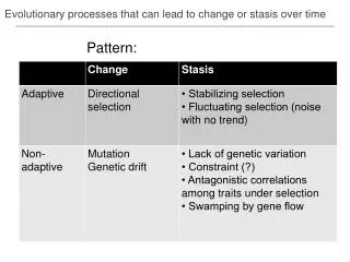
Pattern:
Evolutionary processes that can lead to change or stasis over time. Pattern:. Blomberg ’ s K – measure of phylogenetic signal. phylogenetic signal. low brownian high. K = 0.18. K ~ 1. K = 1.62. Data diagnostics. Blomberg et al. 2003 Evolution examples from Ackerly 2009 PNAS.

Pattern:
E N D
Presentation Transcript
Evolutionary processes that can lead to change or stasis over time Pattern:
Blomberg’s K – measure of phylogenetic signal phylogenetic signal low brownian high K = 0.18 K ~ 1 K = 1.62 Data diagnostics Blomberg et al. 2003 Evolution examples from Ackerly 2009 PNAS
Brownian motion – assumptions and interpretations Evolutionary models
Brownian motion – assumptions and interpretations ∞ -∞ Evolutionary models
Ornstein-Uhlenbeck model (OU-1) the math: brownian motion + ‘rubber band effect’ change is unbounded (in theory), but as rubber band gets stronger, bounds are established in practice repeated movement back towards center erases phylogenetic signal, leading to K << 1 Evolutionary models see Hansen 1997 Evolution Butler and King 2004 Amer. Naturalist
Ornstein-Uhlenbeck model (OU-1) the math: brownian motion + ‘rubber band effect’ change is unbounded (in theory), but as rubber band gets stronger, bounds are established in practice repeated movement back towards center erases phylogenetic signal, leading to K << 1 Evolutionary models see Hansen 1997 Evolution Butler and King 2004 Amer. Naturalist
Ornstein-Uhlenbeck model (OU-2+) the math: brownian motion + ‘rubber band effect’ with different optimal trait values for clades in different selective regimes Balance of stabilizing selection within clades vs. how different the optima are can lead to strong or weak phylogenetic signal This example would be VERY strong signal Evolutionary models see Hansen 1997 Evolution Butler and King 2004 Amer. Naturalist
Early-burst model the math: brownian motion with a declining rate parameter change is unbounded (in theory), but divergence happens rapidly at first and then rates decline and lineages change little divergence among major clades creates high signal: K >> 1 Evolutionary models
Assign proportional weighting of alternative models that best fit data Harmon et al. 2010
1 Var(loge(trait)) million yrs 1 felsen = time Rates of phenotypic diversification under Brownian motion var(x)
Rates of phenotypic diversification under Brownian motion higher rate lower rate time var(x)
rate = 0.015 felsens 0.10 felsens 0.83 felsens Diversification of height in maples, Ceanothus and silverswords ~5.2 Ma ~30 Ma ~45 Ma Ackerly 2009 PNAS Evolutionary rates
North temperate California Hawai’i Rates of phenotypic diversification (estimated for Brownian motion model) Height Leaf size ±1 s.e. Rate (felsens) Acer Acer Aesculus Aesculus lobelioids lobelioids Ceanothus Ceanothus Arbutoideae Arbutoideae silverswords silverswords Ackerly, PNAS in review
time var(x)
Squared change parsimony = ML with BL = 1 Linear parsimony 2.44 0.08 0 2 1.32 1 0.52 0 0.24 0 0.12 0 ML with BL as shown 0.096 2.54 1.6 0.96 0.67 0.56
ML with BL as shown C F E D B A
2 8 6 16 1 6 11 14 8.5 9 11.5 11 19 18 13 12 a b R = 0.74
2 8 6 16 1 6 11 14 8.5 9 11.5 11 19 18 13 12 a 10 8 4 8 3 2 -6 -6 4 12 6 10 10 10 16 15 2 -2 6 5 5 11 13 17 8 6 9 14 b c R = 0.74 R = 0.92
A21223 Fig. 2
1) Assume bivariate normal distribution of variables with = 0 2) Draw samples of 22 and calculate correlation coefficient 3) Repeat 100,000 times! Distribution of correlation coefficients (R) under null hypothesis Crit(R, = 0.05, df = 20) is 0.423 N < -0.423 = 2519; N > 0.423 = 2551 Type I error = 0.051
1) Assume bivariate normal distribution of variables with = 0.5 2) Draw samples of 22 and calculate correlation coefficient 3) Repeat 100,000 times! Crit(R, = 0.05, df = 20) is 0.423 N < -0.423 = 5 N > 0.423 = 68858 Power = 0.69
1) Assume bivariate normal brownian motion evolution along a phylogeny, with ~ 0.0 2) Calculate R using normal correlation coefficient 3) Repeat 10,000 times! Crit(R, = 0.05, df = 20) is 0.423 N < -0.423 = 1050 N > 0.423 = 1044 Type I error = 0.21
1) Assume bivariate normal brownian motion evolution along a phylogeny, with ~ 0.0 2) Calculate R using independent contrasts 3) Repeat 10,000 times! Crit(R, = 0.05, df = 20) is 0.423 N < -0.423 = 246 N > 0.423 = 236 Type I error = 0.048