Understanding Correlation and Regression in Statistical Analysis
Learn about the relationship between variables, strength of correlation, using Pearson’s r for prediction, limitations, covariance, and practical applications in statistics. Explore the significance of models, assumptions, GLM, and more.

Understanding Correlation and Regression in Statistical Analysis
E N D
Presentation Transcript
Correlation and Regression Dharshan Kumaran Hanneke den Ouden
Aims • Is there a relationship between x and y? • What is the strength of this relationship? • Pearson’s r • Can we describe this relationship and use this to predict y from x? • y=ax+b • Is the relationship we have described statistically significant? • ttest • Relevance to SPM • GLM
Relation between x and y • Correlation: is there a relationship between 2 variables? • Regression: how well a certain independent variable predict dependent variable? • CORRELATION CAUSATION • In order to infer causality: manipulate independent variable and observe effect on dependent variable
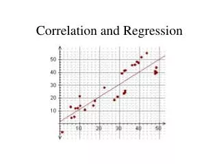
Y X Observation ‘clouds’ Y Y Y Y Y X X Positive correlation Negative correlation No correlation
Covariance ~ DX * DY Variance ~ DX * DX Variance vs Covariance • Do two variables change together?
Covariance • When X and Y : cov (x,y) = pos. • When X and Y : cov (x,y) = neg. • When no constant relationship: cov (x,y) = 0
x ( )( ) - - y - - x x y y x x y y i i i i 0 3 - 3 0 0 2 2 - 1 - 1 1 3 4 0 1 0 4 0 1 - 3 - 3 6 6 3 3 9 å = = 7 y 3 = x 3 Example Covariance What does this number tell us?
Pearson’s R • Covariance does not really tell us anything • Solution: standardise this measure • Pearson’s R: standardise by adding std to equation:
Limitations of r • When r = 1 or r = -1: • We can predict y from x with certainty • all data points are on a straight line: y = ax + b • r is actually • r = true r of whole population • = estimate of r based on data • r is very sensitive to extreme values:
= , predicted value = , true value ε = residual error ε In the real world… • r is never 1 or –1 find best fit of a line in a cloud of observations: Principle of least squares y = ax + b
The relationship between x and y (1) : Finding a and b • Population: • Model: • Solution least squares minimisation:
S2y S2 S2(yi - i) = + 2 2 s s s - ˆ ˆ y y ( ) y y i i What can the model explain? Total variance = predicted variance + error variance 2
predicted variance: 2 predicted Explained variance = total
= + - 2 2 2 2 2 ˆ ˆ s r s ( 1 r ) s y y y = 2 2 2 ˆ s r s ˆ y y s 2 2 2 = ˆ r s s - ˆ ( ) y y y y i i - 2 2 ˆ ( 1 r ) s = y Error variance: 2 Substitute this into equation above
Is the model significant? • We’ve determined the form of the relationship (y = ax + b) and it’s strength (r). Does a prediction based on this model do a better job that just predicting the mean?
= + - 2 2 2 2 2 ˆ ˆ s r s ( 1 r ) s y y y Analogy with ANOVA • Total variance = predicted variance + error variance • In a one-way ANOVA, we have SSTotal = SSBetween + SSWithin
ˆ 2 2 r s y F statistic (for our model) MS Eff = F ( df mod el , dferror ) MSErr MSEff=SSbg/dF MSErr=SSwg/dF /1 - 2 2 / (N-2) ˆ ( 1 r ) s y
F and t statistic - 2 ˆ r ( N 2 ) F = ( df mod el , dferror ) - 2 ˆ 1 r Alternatively (as F is the square of t): - ˆ r ( N 2 ) So all we need to know is N and r!! = t - ( 2 ) N - 2 ˆ 1 r
Basic assumptions • Linear relationship • Homogeneity of variance (Y) • e ~ N(0,s2) • No errors in measurement of X • Independent sampling
e x é ù é ù x é ù y x 1n 12 b1 1 1 11 é ù ê ú ê ú ê ú = + e x x b2 y x ê ú ê ú ê ú ê ú 22 2n 2 21 2 ë û bn ê ú ê ú ê ú e x y x x ë û ë û ë û m1 m m m2 mn SPM- GLM • Y1 = x11b1 +x12b2 +…+ x1nbn + e1 Y2 = x21b1 +x22b2 +…+ x2nbn + e2 : Ym = xm1b1 +xm2b2 +…+ xmnbn+ em . Regression model Multiple regression model In matrix notation
e x é ù é ù x é ù y x 1n 12 b1 1 1 11 é ù ê ú ê ú ê ú = + e x x b2 y x ê ú ê ú ê ú ê ú 22 2n 2 21 2 ë û bn ê ú ê ú ê ú e x y x x ë û ë û ë û m1 m m m2 mn SPM !!!! Observed data = design matrix * parameters + residuals
The End Any questions?* *See Will, Dan and Lucy