CORRELATION AND REGRESSION

1. CORRELATION AND REGRESSION

2. Plan 1. Introduction 2. Types of Correlation 2.1. Positive and Negative Correlation 3. Linear and Non – Linear Correlation 4. The Coefficient of Correlation 4.1. Rank Correlation 5. Regression 5.1. Regression Equation 6. Summary 7. Key words 8. Literature

3. Introduction • So far we have confined our discussion for use in the pharmacy correlation and regression and how to use for solution really task.

4. Types of Correlation • Positive and Negative correlation and • Linear and Non – Linear correlation.

5. Positive and Negative Correlation • If the values of the two variables deviate in the same direction i.e. if an increase (or decrease) in the values of one variable results, on an average, in a corresponding increase (or decrease) in the values of the other variable the correlation is said to be positive.

6. Some examples of series of positive correlation are: • (i) Heights and weights; • (ii) Household income and expenditure; • (iii) Price and supply of commodities; • (iv) Amount of rainfall and yield of crops.

7. Correlation between two variables is said to be negative or inverse if the variables deviate in opposite direction. That is, if the increase in the variables deviate in opposite direction. That is, if increase (or decrease) in the values of one variable results on an average, in corresponding decrease (or increase) in the values of other variable.

8. Some examples of series of negative correlation are: • (i) Volume and pressure of perfect gas; • (ii) Current and resistance [keeping the voltage constant] • (iii) Price and demand of goods.

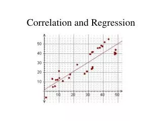
9. Graphs of Positive and Negative correlation: Figure for positive correlation Suppose we are given sets of data relating to heights and weights of students in a class. They can be plotted on the coordinate plane using x – axis to represent heights and y – axis to represent weights. The different graphs shown below illustrate the different types of correlations.

10. Figure for negative correlation

11. Note: (i) If the points are very close to each other, a fairly good amount of correlation can be expected between the two variables. On the other hand if they are widely scattered a poor correlation can be expected between them. (ii) If the points are scattered and they reveal no upward or downward trend as in the case of (d) then we say the variables are uncorrelated. (iii) If there is an upward trend rising from the lower left hand corner and going upward to the upper right hand corner, the correlation obtained from the graph is said to be positive. Also, if there is a downward trend from the upper left hand corner the correlation obtained is said to be negative. (iv) The graphs shown above are generally termed as scatter diagrams. Note:

12. Example:1 • The following are the heights and weights of 15 students of a class. Draw a graph to indicate whether the correlation is negative or positive.

13. Since the points are dense (close to each other) we can expect a high degree of correlation between the series of heights and weights. Further, since the points reveal an upward trend, the correlation is positive. Arrange the data in increasing order of height and check that , as height increases, the weight also increases, except for some (stray) cases..

14. Linear And Non – Linear Correlation The correlation between two variables is said to be linear if the change of one unit in one variable result in the corresponding change in the other variable over the entire range of values. For example consider the following data.

15. Thus, for a unit change in the value of x, there is a constant change in the corresponding values of y and the above data can be expressed by the relation • y = 3x +1 • In general two variables x and y are said to be linearly related, if there exists a relationship of the form • y = a + bx • where ‘a’ and ‘b’ are real numbers. This is nothing but a straight line when plotted on a graph sheet with different values of x and y and for constant values of a and b. Such relations generally occur in physical sciences but are rarely encountered in economic and social sciences.

16. The relationship between two variables is said to be non – linear if corresponding to a unit change in one variable, the other variable does not change at a constant rate but changes at a fluctuating rate. In such cases, if the data is plotted on a graph sheet we will not get a straight line curve. For example, one may have a relation of the form • y = a + bx + cx2 • or more general polynomial.

17. The Coefficient of Correlation • One of the most widely used statistics is the coefficient of correlation‘r’ which measures the degree of association between the two values of related variables given in the data set. It takes values from + 1 to – 1. If two sets or data have r = +1, they are said to be perfectly correlated positively if r = -1 they are said to be perfectly correlated negatively; and if r = 0 they are uncorrelated. • The coefficient of correlation ‘r’ is given by the formula

18. Example:2: • A study was conducted to find whether there is any relationship between the weight and blood pressure of an individual. The following set of data was arrived at from a clinical study. Let us determine the coefficient of correlation for this set of data. The first column represents the serial number and the second and third columns represent the weight and blood pressure of each patient.

19. Solution:

20. Rank Correlation • Data which are arranged in numerical order, usually from largest to smallest and numbered 1,2,3 ---- are said to be in ranks or ranked data.. These ranks prove useful at certain times when two or more values of one variable are the same. The coefficient of correlation for such type of data is given by Spearman rank difference correlation coefficient and is denoted by R. • In order to calculate R, we arrange data in ranks computing the difference in rank ‘d’ for each pair. The following example will explain the • usefulness of R. R is given by the formula

21. Example:3 • The data given below are obtained from student records. Calculate the rank correlation coefficient ‘R’ for the data. • Note that in the G. P. A. column we have two students having a grade point average of 8.6 also in G. R. E. score there is a tie for 2000.

22. Now we first arrange the data in descending order and then rank • 1,2,3,---- 10 accordingly. In case of a tie, the rank of each tied value is the mean of all positions they occupy. In x, for instance, 8.6 occupy ranks 5 and 6. So each has a rank Similarly in ‘y’ 2000 occupies ranks 9 and 10, so each has rank

23. Now we come back to our formula • We compute ‘d’ , square it and substitute its value in the formula.

24. So here, n = 10, sum of d2 = 12. So Note: If we are provided with only ranks without giving the values of x and y we can still find Spearman rank difference correlation R by taking the difference of the ranks and proceeding in the above shown manner.

25. Regression • If two variables are significantly correlated, and if there is some theoretical basis for doing so, it is possible to predict values of one variable from the other. This observation leads to a very important concept known as • ‘Regression Analysis’. • Regression analysis, in general sense, means the estimation or prediction of the unknown value of one variable from the known value of the other variable. It is one of the most important statistical tools which is extensively used in almost all sciences – Natural, Social and Physical. It is specially used in business and economics to study the relationship between two or more variables that are related causally and for the estimation of demand and supply graphs, cost functions, production and consumption functions and so on. • Regression analysis was explained by M. M. Blair as follows: “Regression analysis is a mathematical measure of the average relationship between two or more variables in terms of the original units of the data.”

26. Regression Equation • Suppose we have a sample of size ‘n’ and it has two sets of measures, denoted by x and y. We can predict the values of ‘y’ given the values of ‘x’ by using the equation, called the REGRESSION EQUATION. • y* = a + bx • where the coefficients a and b are given by • The symbol y* refers to the predicted value of y from a given value of x from the regression equation.

27. Example: 4 • Scores made by students in a statistics class in the mid - term and final examination are given here. Develop a regression equation which may be used to predict final examination scores from the mid – term score.

28. Solution: • We want to predict the final exam scores from the mid term scores. So let us designate ‘y’ for the final exam scores and ‘x’ for the mid – term exam scores. We open the following table for the calculations.

29. Numerator of b = 10 * 65,071 – 785 * 810 = 6,50,710 – 6,35,850 = 14,860 • Denominator of b = 10 * 64, 521 – (785)2 = 6,45,210 – 6,16,225 = 28,985 • Therefore, b = 14,860 / 28,985 = 0.5127 • Numerator of a = 810 – 785 * 0.5127 = 810 – 402.4695 = 407.5305 • Denominator of a = 10 • Therefore a = 40.7531 • Thus , the regression equation is given by y* = 40.7531 + (0.5127) x • We can use this to find the projected or estimated final scores of the students. • For example, for the midterm score of 50 the projected final score is y* = 40.7531 + (0.5127) 50 = 40.7531 + 25.635 = 66.3881 which is a quite a good estimation. • To give another example, consider the midterm score of 70. Then the projected final score is • y* = 40.7531 + (0.5127) 70 = 40.7531 + 35.889 = 76.6421, which is again a very good estimation. • This brings us to the end of this chapter. We close with some problems for you.

30. Summary • Correlation does not mean causation • Even if two variables exhibit very strong • correlation, they may be completely • independent of each other • Statistics is nice and a great tool, but it • cannot replace thinking

31. KEY WORDS • coefficient of Determination: It is equal to the square ofthe correlation coefficient. • Corklation : It is a quantitative measure of the strength of therelationship that may exist among certain variables. • Cross Section Data : In cross section data, we have observations for avariable for different units at the same point of time. • Econometrics : It is described as the application of statistical tools inthe quantitative analysis of economic phenomena. • Mathematical Model : The mathematical form of some economic theory iswhat is generally called a mathematical model. • Method of Least Square : 1t is the method of estimating the parameters of aregression equation in such a fashion that the sum ofthe squares of the differences between the actualvalues or observed values of the dependent variableand their estimated values from the regressionequation is minimum. • Multiple Regression : It is a regression equation with more than oneindependent variable.

32. Nonsense Correlation : The presence of correlation between twovariables when there does not exist any meanmgfdrelationship between them is known as nonsense • correlation. • Pooled Data : In pooled data, we have time series observationsfor various cross sectional units. Here, we combinethe element oftime series with that of cross sectiondata. • Regression Equation : It is the equation that specifies the relationshipbetween the dependent and the independentvariables for the purpose of estimating the constantsor the parameters of the equation with the help ofempirical data on the variables. • Regression : It is a statistical analysis of the nature of therelationship between the dependent and theindependent variables. • Reverse Regression : It is an independent estimation of a new regressionequation when the independent variable ofthe origunalequation is changed into the dependent variable and • the dependent variable of the original equation ischanged into the independent variable.

33. Literature: • Gujrati, Damodar N. (2003); Basic Econometrics, Fourth Edition, Chapter 2, • Chapter 3, and Chapter 7, McGraw-Hill, New York. • Maddala, G.S. (2002); Introduction to Econometrics, Third Edition, Chapter 3and Chapter 4, John Wiley & Sons Ltd., West Sussex. • Pindyck, Robert S. and Rubinfeld, Daniel L. (1 991), Econometric Models andEconomic Forecasts, Third Edition, Chapter 1; McGraw-Hill, New York. • Karmel, P.H. and Polasek, M. (1 986); AppliedStatistics for Economists, FourthEdition, Chapter 8, Khosla Publishing House, Delhi.

34. Good Luck