Download
1 / 15
160 likes | 693 Views
Discrete probability distributions . Chapter 5 . Outline. Section 5-1: Introduction Section 5-2: Probability Distributions Section 5-3: Mean, Variance, Standard Deviation and Expectation Section 5-4: The Binomial Distribution Section 5-5: Summary. Section 5-1 Introduction. Overview.

E N D
Discrete probability distributions Chapter 5
Outline • Section 5-1: Introduction • Section 5-2: Probability Distributions • Section 5-3: Mean, Variance, Standard Deviation and Expectation • Section 5-4: The Binomial Distribution • Section 5-5: Summary
Overview • This chapter will deal with the construction of discrete probability distributions by combining methods of descriptive statistics from Chapters 2 and 3 and those of probability presented in Chapter 4. • A probability distribution, in general, will describe what will probably happen instead of what actually did happen
Combining Descriptive Methods and Probabilities In this chapter we will construct probability distributions by presenting possible outcomes along with the relative frequencies we expect.
Why do we need probability distributions? • Many decisions in business, insurance, and other real-life situations are made by assigning probabilities to all possible outcomes pertaining to the situation and then evaluating the results • Saleswoman can compute probability that she will make 0, 1, 2, or 3 or more sales in a single day. Then, she would be able to compute the average number of sales she makes per week, and if she is working on commission, she will be able to approximate her weekly income over a period of time.
Section 5-2 Probability Distributions Objective: Construct a probability distribution for a random variable
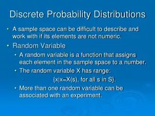
Remember • From Chapter 1, a variable is a characteristic or attribute that can assume different values • Represented by various letters of the alphabet • From Chapter 1, a random variable is a variable whose values are determined by chance • Typically assume values of 0,1,2…n
Remember Discrete Variables (Data)— Chapter 5 Continuous Variables (Data)---Chapter 6 • Can be assigned values such as 0, 1, 2, 3 • “Countable” • Examples: • Number of children • Number of credit cards • Number of calls received by switchboard • Number of students • Can assume an infinite number of values between any two specific values • Obtained by measuring • Often include fractions and decimals • Examples: • Temperature • Height • Weight • Time
Examples: State whether the variable is discrete or continuous • The height of a randomly selected giraffe living in Kenya • The number of bald eagles located in New York State • The exact time it takes to evaluate 27 + 72 • The number of textbook authors now sitting at a computer • The exact life span of a kitten • The number of statistics students now reading a book • The weight of a feather
Discrete Probability Distribution • Consists of the values a random variable can assume and the corresponding probabilities of the values. • The probabilities are determined theoretically or by observation • Can be shown by using a graph (probability histogram), table, or formula • Two requirements: • The sum of the probabilities of all the events in the sample space must equal 1; that is, SP(x) = 1 • The probability of each event in the sample space must be between or equal to 0 and 1. That is, 0 < P(x) < 1
Example: Determine whether the distribution represents a probability distribution. If it does not, state why.
Example: Determine whether the distribution represents a probability distribution. If it does not, state why. • A researcher reports that when groups of four children are randomly selected from a population of couples meeting certain criteria, the probability distribution for the number of girls is given in the accompanying table
Example: Construct a probability distribution for the data • Based on past results found in the Information Please Almanac, there is a 0.1818 probability that a baseball World Series contest will last four games, a 0.2121 probability it will last five games, a 0.2323 probability that it will last six games, and a 0.3737 probability that it will last seven games. • In a study of brand recognition of Sony, groups of four consumers are interviewed. If x is the number of people in the group who recognize the Sony brand name, then x can be 0, 1, 2, 3, or 4 and the corresponding probabilities are 0.0016,0.0564, 0.1432, 0.3892, and 0.4096
Assignment Page 250 #7-27 odd (no graphs on #19-27 odd)