Download
1 / 30
340 likes | 641 Views
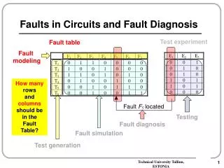
F. F. F. F. F. F. F. 1. 2. 3. 4. 5. 6. 7. T. 0. 1. 1. 0. 0. 0. 0. 1. T. 1. 0. 0. 1. 0. 0. 0. 2. T. 1. 1. 0. 1. 0. 1. 0. 3. T. 0. 1. 0. 0. 1. 0. 0. 4. T. 0. 0. 1. 5. Faults in Circuits and Fault Diagnosis. Test experiment. F ault table.

E N D
F F F F F F F 1 2 3 4 5 6 7 T 0 1 1 0 0 0 0 1 T 1 0 0 1 0 0 0 2 T 1 1 0 1 0 1 0 3 T 0 1 0 0 1 0 0 4 T 0 0 1 5 Faults in Circuits and Fault Diagnosis Test experiment Fault table Fault modeling How many rows and columns should be in the Fault Table? 0 1 1 0 T 0 0 1 0 0 1 1 6 Fault F located 5 Testing Fault diagnosis Fault simulation Test generation
Sequential Fault Diagnosis Sequential fault diagnosis by Edge-Pin Testing Diagnostic tree: Two faults F1,F4remain indistinguishable Not all test patterns used in the fault table are needed Different faults need for identifying test sequences with different lengths The shortest test contains two patterns, the longest four patterns
Stuck-at Faults and their Properties Fault equivalence and fault dominance: A B C D Fault class 1 1 1 0 A/0, B/0, C/0, D/1Equivalence class 0 1 1 1 A/1, D/0 1 0 1 1 B/1, D/0 Dominance classes 1 1 0 1 C/1, D/0 A & D B C Fault collapsing: 1 1 Dominance 1 0 1 & & 1 1 & & 1 0 0 Dominance Equivalence Equivalence
& & & Gate-Level Test Generation • Fault sensitisation: • x7,1= D • Fault propagation: • x2=1, x1=1, b =1, c =1 • Line justification: • x7= D = 0: x3= 1, x4= 1 • b = 1: (already justified) • c = 1: (already justified) Single path fault propagation: 1 1 Macro 1 d 1 1 a & 2 D & 71 D D 1 & e 3 7 72 b 1 1 4 y D D & 5 73 c 1 6 Test pattern Symbolic fault modeling: D = 0 - if fault is missing D = 1 - if fault is present
Boolean derivatives Boolean function: Y = F(x) = F(x1, x2, … , xn) Boolean partial derivative:
Boolean Derivatives Useful properties of Boolean derivatives: These properties allow to simplify the Boolean differential equation to be solved for generating test pattern for a fault at xi IfF(x)is independentofxi Näide:
Calculation of Boolean Derivatives Given: Calculation of the Boolean derivative:
Derivatives for complex functions Boolean derivative for a complex function: Example: Additional condition:
Generalization: Functional Fault Model Constraints: Component with defect: Fault model: (dy,Wd), (dy,{Wkd}) Component F(x1,x2,…,xn) y Wd Fault-free Faulty Constraints calculation: Defect Logical constraints d = 1, if the defect is present
Mapping Transistor Faults to Logic Level A transistor fault causes a change in a logic function not representable by SAF model Function: y Faulty function: x1 x4 0 – defect d is missing 1 – defect d is present Short d= Defect variable: x2 Generic function with defect: x5 x3 Mapping the physical defect onto the logic level by solving the equation:
Mapping Transistor Faults to Logic Level Function: Faulty function: Generic function with defect: y x1 x4 Short Test calculation by Boolean derivative: x2 x5 x3
Deductive Fault Simulation with BDs Macro-level fault propagation: Fault list calculated: 1 1 Ly = (L1 L2) - (L3 (L4 L5)) b & 1 1 2 1 1 y 0 0 3 B & A 0 0 c 4 1 0 a 5 Solving Boolean differential equation: A B Lk A B
Boolean Differentials and FaultDiagnosis Diagnostic experiment: Substitution of values: x1 = 0 x2 = 1 x3 = 1 dy = 0 Test pattern - Correct reaction Adjusting for SAF faults: Partial diagnosis:
Boolean Differentials and FaultDiagnosis 1) Correct output signal: Two diagnostic experiments: x1 = 0 x2 = 1 x3 = 1 dy = 0 2) Erroneous output signal: x1 = 0 x2 = 0 x3 = 0 dy = 1 Diagnosis from two experiments:
Boolean Differentials and FaultDiagnosis Diagnosis from two experiments: = 0 Final diagnosis: Rule: Rule: The linex3works correctly There is a fault: The fault is missing
BDDs and Testing of Logic Circuits Path activation Correct y y 1 Fault signal x x 1 1 1 1 activation 0 0 x 1 1 x x x x x ® 1 0 2 2 2 3 3 x = 1 1 3 y 0 x 4 x x x x x 4 4 5 5 5 Error 0 ( ) F X x 0 6 Fault x 7 Stuck - at - 0 x x x x 6 6 7 7 0 How about testing the internal nodes of the circuit? SSBDD By the BDD for F(X) we can generate test patterns only for testing inputs 0 0 • The tasks on BDDs: • Pattern simulation (analysis) • Pattern generation (synthesis)
BDDs and Test Generation Structural BDD: x110 Test generation for: Test generation for: 1 1 x11 x21 1 y x11 10 x1 x21 x10 1 & x2 10 10 x12 x31 x4 x12 10 x31 0 0 x3 y & 1 0 x4 Functional BDD: x22 x32 0 x13 & x13 1 1 & y x2 1 x1 x22 0 1 0 x32 10 Test pattern: x1 x2 x3 x4 y 1 10- x4 x3 x2 ALGORITHM: Begin TG with Functional BDD Simulate the test on Structural BDD Update the test on Structural BDD 1 0
Example: Test Generation with SSBDDs Testing Stuck-at-1 faults on paths: y x21 x11 1 x11 x1 x21 & x2 x31 x4 x12 x12 1 x31 x3 y & 1 x4 x22 x32 x13 1 Test pattern: & x13 x1 x2 x3 x4 y 00110 & x22 0 x32 Tested faults: x121, x221 Not tested: x111
Test Pairs for Multiple Fault Testing Testing of multiple faults by pairs of patterns To test a path under any multiple faults, two pattern test is needed Tested path for b 1/0 11 00 a & 01 No error b 11/11 & b 1 00/11 01/00 The lower path from b is under test A pair of patterns is applied on b There is a masking fault c 1 & c 1 01 Error & 00 11 10/11 c & 11 d 11/00 1st pattern: fault b1 is masked 2nd pattern: fault c1 is detected Either the fault on the path is detected or the masking fault is detected
Test Pair is not Detecting the Fault Tested path for b 1/0 11 00 a & 01 Test pair is not correct b 11/11 & b 1 00/11 d 01/01 & c 1 01 No error detected & 01 11 10/10 c & 10 11/11 Test pair is not systematic – more than one variable is changing the value 1st pattern: fault b1 is masked 2nd pattern: fault c1 is masked
Fault Analysis with SSBDDs Algorithm: • Determine the activated path to find the fault candidates • Analyze the detectability of the each candidate fault (each node represents a subset of real faults) y x21 x11 x11 0 x1 x21 1 1 & x31 x4 x12 x2 1 x12 0 0 0 x31 x3 y & 1 x22 x32 x13 x4 & x13 0 0 & 0 1 x22 x32 0
Synthesis of Functional HLDDs Results of cycle based symbolic simulation: Data Flow Diagram/FSMD q = 0 Begin q = 1 A = B + C 1 0 x A q = 2 q = 4 A = A + 1 B = B + C 1 0 0 1 x x A B q = 3 C = C B = B C = C 0 1 0 1 x x C C A = C + B A = A + B + C C = A + B q = 5 END
Synthesis of HLDDs Extraction of the behaviour for A: Results of symbolic simulation: Predicate equation for A: A =f (q, A, B, C, xA, xC) = = (q=0)(B+C) (q=1)(xA=0) (A + 1) (q=3)(xC=1)( C+B) (q=4)(xA=0)(xC=0)(A+ B + C + 1)
Synthesis of HLDDs Decision diagram for A: Extraction of the behaviour for A: Predicate equation for A: A = (q=0)(B+C) (q=1)(xA=0) (A + 1) (q=3)(xC=1)( C+B) (q=4)(xA=0)(xC=0)(A+ B + C + 1) Synthesis method: similar to Shannon’s expansion theorem:
R 2 0 y # 0 4 1 R 2 M1 0 0 2 y y R + R 3 1 1 2 R2 1 IN + R 2 1 IN 2 R 1 3 0 y R * R 2 R2 +M3 1 2 1 IN* R 2 M2 High-Level Decision Diagrams Superposition of High-Level DDs: A single DD for a subcircuit Instead of simulating all the components in the circuit, only a single path in the DD should be traced
y y y y 1 2 3 4 a R · c 1 M + 1 e · M R 3 2 b · * M · 2 IN · d Test Generation for Digital Systems High-level test generation with DDs: Conformity test Decision Diagram Multiple paths activation in a single DD Control function y3 is tested R 2 0 y # 0 4 Data path 1 R 2 0 0 2 y y R + R 3 1 1 2 1 IN + R 2 1 IN 2 R 1 3 0 y R * R 2 1 2 1 IN* R Control: For D = 0,1,2,3: y1 y2 y3 y4 = 00D2 Data: Solution of R1+ R1 IN R1 R1* R1 Test program: 2
y y y y 1 2 3 4 a R · c 1 M + 1 e · M R 3 2 b · * M · 2 IN · d Test Generation for Digital Systems High-level test generation with DDs: Scanning test Decision Diagram Single path activation in a single DD Data function R1* R2is tested R 2 0 y # 0 4 Data path 1 R 2 0 0 2 y y R + R 3 1 1 2 1 IN + R 2 1 IN 2 R 1 3 0 y R * R 2 1 2 1 IN* R Control: y1 y2 y3 y4 = 0032 Data: For all specified pairs of (R1, R2) Test program: 2
I1: MVI A,D A IN I2: MOV R,A R A I3: MOV M,R OUT R I4: MOV M,A OUT IA I5: MOV R,M R IN I6: MOV A,M A IN I7: ADD R A A + R I8: ORA R A A R I9: ANA R A A R I10: CMA A,D A A Decision Diagrams for Microprocessors DD-model of the microprocessor: Instruction set: 1,6 A I IN 3 2,3,4,5 I R OUT IN 4 7 A + R A 8 2 A R I A R 9 A R 5 IN 10 A 1,3,4,6-10 R
Decision Diagrams for Microprocessors High-Level DD-based structureofthe microprocessor (example): DD-model of the microprocessor: 1,6 IN A I IN R 3 2,3,4,5 I R OUT A 4 I 7 A + R OUT A 8 2 A R I A R 9 A A R 5 IN 10 A + R A 1,3,4,6-10 R
Test Program Synthesis for Microprocessors Scanning test program for adder: Instruction sequence T = I5 (R)I1 (A)I7 I4 for all needed pairs of (A,R) • Test program: • For j=1,n • Begin • I5: Load R = IN(j1) • I1: Load A = IN(j2) • I7: ADD A = A + R • I4: Read A • End I4 OUT I7 A I1 A R IN(2) I5 R IN(1) IN(j2) A IN(j1) Time: t t - 1 t - 2 t - 3 Observation Test Load Test data Test results