Download
1 / 62
630 likes | 721 Views
Explore the fascinating world of Kellet’s whelk, Kelletia kelletii, including its habitat, feeding habits, breeding season, and economic significance. Discover its genetic diversity, population genetics study, and expansion since 1980. Learn about the species' genetic isolation and dispersal connectivity. Unravel the correlation between genetic distance and geographic location, shedding light on regional equilibrium and non-equilibrium dynamics. Dive into the interplay of gene flow and genetic drift, and the impact of regional disturbances on population structure. Delve into the intricate patterns of genetic variation and connectivity in Kellet’s whelk populations, offering insights into their evolution and conservation.

E N D
17 cm 6 mm
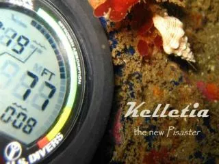
Kellet’s whelk, Kelletia kelletii Habitat: Rocky reef/kelp forests. Partial migration offshore during winter? Carnivorous predator and scavenger. Radula at end of feeding proboscis used to drill through animal shells (e.g., snails, bivalves, etc.) and excavate concealed prey (e.g., tube worms).
Kellet’s whelk, Kelletia kelletii Preyed upon by… Sea otters Lobster? Elasmobranchs (bat ray, sharks)?? Their shell is remarkably thick!
Kellet’s whelk, Kelletia kelletii Spring/summer breeding season. Mating & internal fertilization. Females lay 100+ egg capsules/year. Capsule = 1000+ eggs. Larvae (veliger) hatch out of capsules after 30 days. Lecithotropic veliger in plankton for 45 days (?). Mean Dd ~ 90 km (Siegel et al. 2003; U = 0) Settlement cue not known. Reproductively mature after ~6 years?
Juveniles: Found in highly varying densities and across a wide range of depth gradients within the nearshore system.
Economic value: Excellent for lawn art (match gnomes beautifully!)
Economic value: Focus of developing fishery (by-catch in lobster traps) Sold to US domestic Asian market (mostly in LA) Mean price = $1.43/kg = ~$0.15/whelk Aseltine-Neilson et al. 2006
Expansion since ~1980 RANGE Bahia Asuncion
Density: mainland > islands. Baja highest. Northern Channel Islands Catalina Island (southern)
POPULATION GENETICS STUDY COI: Cytochrome Oxidase I gene in mtDNA mtDNA: circular, ~16K basepairs long COI sequence: 528 basepairs long One sequence per individual adult N = 15 – 35 samples/site N = 16 sites, spanning entire range COI
COI sampling sites Expansion since ~1980 Bahia Asuncion
Site Hap diversity MA 0.9076 WC 0.9048 DC 0.9191 HR 0.9181 RR 0.8807 GI 0.8762 YB 0.7664 NR 0.8246 IV 0.8840 SV 0.7966 PV 0.8891 DP 0.9025 PL 0.8723 SQ 0.8123 TT 0.7277 BA 0.8303 Expansion since ~1980 Bahia Asuncion
Regionwide genetic structure statistics Analysis of Molecular Variance (AMOVA): Fst = 0.012 (P = 0.001) Pairwise differences between sites: Fst range: 0.02 – 0.05 (P < 0.05) Bonferroni: (120 pairs)(0.05) = 6 expected by chance. 19 found. Spatial Analysis of Molecular Variance (SAMOVA): Fst = 0.02 – 0.03 (P = 0.002)
Genetic isolation by geographic distance: what to expect No correlation Non-equilibrium No correlation? stirred Positive correlation Stepping stone Equilibrium
Regional equilibrium Expanded range Regional equilibrium Expanded range Regional non-equilibrium Relative dominance of gene flow vs. genetic drift varies with scale At large scales, drift > Expansion, followed by isolation (Hutchinson & Templeton 1999)
Genetic isolation by geographic distance: what to expect IBD signal only present at small scales Non-equilibrium stirred Stepping stone Periodic regional disturbance due to el Nino Equilibrium
Fst = 0.0041*Ln(distance) – 0.0112 R2 = 0.07
12 km site aggregate Pairwise Fst Kij dispersal connectivity
1 MA 2 DC 3 HR 4 RR 5 GI 6 YB 7 IV 8 SV 9 PV 10 DP 11 PL 12 SQ 13 TT 14 BA
1 MA 2 DC 3 HR 4 RR 5 GI 6 YB 7 IV 8 SV 9 PV 10 DP 11 PL 12 SQ 13 TT 14 BA Fst = 0.03 (P = 0.001)
June 2000 SST (Ocean Data Center, UCSC) TT BA
1 MA 2 DC 3 HR 4 RR 5 GI 6 YB 7 IV 8 SV 9 PV 10 DP 11 PL 12 SQ 13 TT 14 BA Fst = 0.03 (P = 0.001)
1 MA 2 DC 3 HR 4 RR 5 GI 6 YB 7 IV 8 SV 9 PV 10 DP 11 PL 12 SQ 13 TT 14 BA Fst = 0.014 (P = 0.001)
1 MA 2 DC 3 HR 4 RR 5 GI 6 YB 7 IV 8 SV 9 PV 10 DP 11 PL 12 SQ 13 TT 14 BA Fst = 0.013 (P = 0.001)
Density: mainland > islands. Baja highest. Northern Channel Islands Catalina Island (southern)