Download
1 / 36
450 likes | 1.07k Views
Chapter 7 Differentiation and Integration. Finite-difference differentiation. Example: Evaporation Rates. Table: Saturation Vapor Pressure ( e s ) in mm Hg as a Function of Temperature ( T ) in °C. The slope of the saturation vapor pressure curve at 22 °C (3 methods) :

E N D
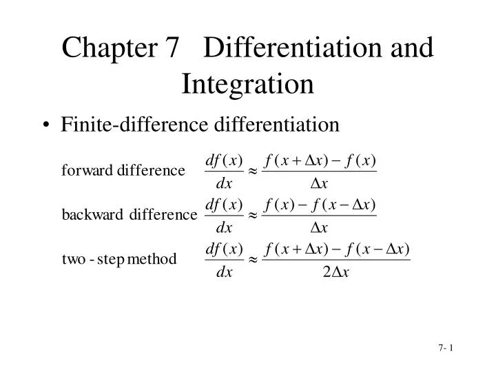
Chapter 7 Differentiation and Integration • Finite-difference differentiation
Example: Evaporation Rates Table: Saturation Vapor Pressure (es) in mm Hg as a Function of Temperature (T) in°C
The slope of the saturation vapor pressure curve at 22°C (3 methods) : The true value is 1.20 mm Hg/°C, so the two-step method provides the most accurate estimate.
Differentiation Using a Finite-difference Table Example: Finite-difference Table for Specific Enthalpy (h) in Btu/lb and Temperature (T) in ºF
For example, at a temperature of 1200 ºF, the forward, backward, and two-step methods yield: • The rate of change of cp at T= 1200 ºF is
Differentiating an Interpolating Polynomial The derivative: Gregory-Newton interpolation polynomial: It is more difficult to evaluate the derivative:
The second-order approximation: The second-order approximation of the first derivative with forward difference:
The second-order approximation of the second derivative with forward difference: • The first-order and second-order approximation of the first derivative with backward difference:
The first-order and second-order approximation of the second derivative with backward difference: • How to derive (for reference only)
The first-order and second-order approximation of the first derivative with the two-step method: • The first-order and second-order approximation of second derivative with the two-step method:
Example: Evaporation Rates Second-order with forward, backward, two-step: The true value at T = 22ºC is 1.2 mm Hg/ºC
Numerical Integration • The area under the curve f(x) between x=a and x=b: • Example: the volume rate of flow (Q) of water in a channel or through a pipe is the integral of the velocity (V) and the incremental area (dA):
Interpolation Formula Approach The Gregory-Newton interpolation polynomial:
Another way to get the trapezoidal formula The linear polynomial passing the data points:
The absolute value of the upper bound on the error for the Trapezoidal rule is:
Example: Trapezoidal Rule for Integration • n = 4 • The trapezoidal rule provides
Example: Flow Rate • The flow rate (Q) of an incompressible fluid is given by the integral. in which V is the velocity and A is the area. • For a circular pipe of radius r, the incremental area dA is equal to 2πrdr.
Table 6: The Data for Estimating the Flow Rate of a Fluid in a Circular Piple
For a pipe of diameter of 1 ft trapezoidal rule:
Simpson’s Rule • Simpson’s rule: where • Simpson’s rule can only be applied when there are an even number of subintervals:
Proof of Simpson’s Rule Using a second-order polynomial:
Passing through the three data points: Then, we can obtain the Simpson’s formula.
The absolute value of the upper bound on the error for the Simpson’s rule is estimated by
Example: Flow Rate Problem • Applying Simpson’s rule to the data of Table.6
Romberg Integration • Denoting the trapezoidal estimate as I01 where a and b are the start and end of an interval. • A second estimate I11:
A third estimate I21 can be obtained using three equally spaced intermediate points m1, m2, and m3 and it can be rewritten as
Continuing this subdividing of the interval leads to the following recursive relationship • The general extrapolation formula in recursive form is
The values of Iij can be presented in the following upper-triangular matrix form:
Example: Romberg Method for Integration • For the function f(u) = ueku, the integral is • Let k = 2, we want to calculate The true value of the integral is 2.097264 (seven significant digits).
Similarly for i = 5, I51=2.09899 • I02 is computed as following: • I03 is computed as following: • The Romberg method yields an exact value to six significant digits for the integral of 2.09726