Download

1 / 9
90 likes | 299 Views
Mathematics Roots, Differentiation and Integration. Prof. Muhammad Saeed. Roots. r = roots(p) r = fzero (func,x0), r = fzero ( func ,[x1 x2]) r = fzero ('3*x^3+2*x^2-5*x+7',5) r = fzero (@myfun,x0) r = fzero (@(x) exp(x)*sin(x),x0) Hfnc = @(x) x^2* cos (2*x)*sin(x*x)

E N D
MathematicsRoots, Differentiation and Integration Prof. Muhammad Saeed
Roots • r = roots(p) • r = fzero(func,x0), • r = fzero(func,[x1 x2]) • r = fzero('3*x^3+2*x^2-5*x+7',5) • r = fzero(@myfun,x0) • r = fzero(@(x) exp(x)*sin(x),x0) • Hfnc = @(x) x^2*cos(2*x)*sin(x*x) • r = fzero(Hfnc, [x0 x1]) • 4. a= 1.5; r = fzero(@(x) myfun(x,a),0.1) • 5. options = optimset('Display','iter','TolFun',1e-8) • opts=optimset(options,'TolX',1e-4) • r = fzero(fun,x0,opts) Mathematical modeling & Simulations
6. [r,fval] = fzero(...) • 7. [r,fval,exitflag] = fzero(...) • 8. [r,fval,exitflag,output] = fzero(...) • output.algorithm : Algorithm used • output.funcCount Number of function evaluations • output.intervaliterations: Number of iterations taken to find an interval • output.iterations: Number of zero-finding iterations • output.message: Exit message • ExitFlags • 1 Function converged to a solution x. • -1 Algorithm was terminated by the output function. • -3 NaN or Inf function value was encountered during search for an interval containing a sign change. • -4 Complex function value was encountered during search for an interval containing a sign change. • -5 Algorithm might have converged to a singular point. • 9.[….. ] =fminbnd(…) Mathematical modeling & Simulations
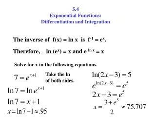
Residues [r,p,k] = residue(b,a)[b,a] = residue(r,p,k) • Integration • Symbolic • a.syms x t z alpha; • # int(-2*x/(1+x^2)^2) • # int(x/(1+z^2),z) • # int(x*log(1+x),0,1) • # int(2*x, sin(t), 1) Mathematical modeling & Simulations
Integration • Numerical • # Z = trapz(Y)# Z = trapz(X,Y)Example: IntegralTrapz.m • # Z = quad(hfun,a,b)# Z = quad(hfun,a,b,tol)# [Z,fcnt] = quad(...) • # Z= quad(@fun,a,b) • # [Z, fcnt]=quad(……) • # Z=quad(fun,a,b,tol,trace) • # Z=quadl(……..) • “The quad function may be most efficient for low accuracies with • nonsmooth integrands. The quadl function may be more efficient • than quad at higher accuracies with smooth integrands.” Mathematical modeling & Simulations
Integration q = quadgk(fun,a,b)[q,errbnd] = quadgk(fun,a,b,tol)[q,errbnd] = quadgk(fun,a,b,param1,val1,param2,val2,...) [q,errbnd] = quadgk(@(x)x.^5.*exp(-x).*sin(x),0,inf, 'RelTol',1e-8,'AbsTol',1e-12) “The ‘quadgk’ function may be most efficient for high accuracies and oscillatory integrands. It supports infinite intervals and can handle moderate singularities at the endpoints. It also supports contour integration along piecewise linear paths.” q = dblquad(fun,xmin,xmax,ymin,ymax)q = dblquad(fun,xmin,xmax,ymin,ymax,tol)q = dblquad(fun,xmin,xmax,ymin,ymax,tol,method) q = dblquad(@(x,y)sqrt(max(1-(x.^2+y.^2),0)), -1, 1, -1, 1) triplequad(fun,xmin,xmax,ymin,ymax,zmin,zmax)triplequad(fun,xmin,xmax,ymin,ymax,zmin,zmax,tol)triplequad(fun,xmin,xmax,ymin,ymax,zmin,zmax,tol,method) F = @(x,y,z)y*sin(x)+z*cos(x); Q = triplequad(F,0,pi,0,1,-1,1);
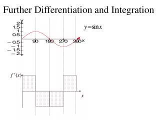
Differentiation • Symbolic • syms x • f = sin(5*x) • g = exp(x)*cos(x); diff(g); diff(g,2) • syms s t • f = sin(s*t) ; • diff(f,t) ; • diff(f,s); • diff(f,t,2); • Numerical • diff(x) ; diff(y) • z=diff(y)./diff(x) • z=diff(y,2)./diff(x,2) • polyder(p) • polyder(a,b) Mathematical modeling & Simulations
Rounding • ceil • floor • fix • round • Discrete Mathematics • fs=factor(n) • f=factorial(n) • g=gcd(a,b) • l=lcm(a,b) • c=nchoosek(n,r) • v=[3 6 7]; p=perms(v) • p=primes(n) Mathematical modeling & Simulations
END Mathematical modeling & Simulations