Download

1 / 21
210 likes | 250 Views
Explore economic models derived from theories and econometric models estimated from data using Greek characters for parameters. Learn about variables, endogenous and exogenous variables, simultaneous equation models, structural and reduced form models, and more in this comprehensive guide to economic and econometric modeling.

E N D
Economic and Econometric Models • The model of the economic behaviour that has been derived fro a theory is the economic model • After the unknown parameters have been estimated by using economic data foe the variables and by using an appropriate econometric estimation method, one has obtained an econometric model. • It is common to use greek characters to denote the parameters. • C=f(Y) economic model • C=β1 + β2 Y , C=15.4+0.81Y econometric model
Economic data • Time series data, historical data • Cross sectional data • Panel data Variables of an economic model Dependent variable Independet variable, explanatory variable, control variable The nature of economic variables can be endogeneous , exogeneous or lagged dependent
A variable is an endogenous variable if the variable is dtermined in the model. Therefore dependant variable is always an endogenous variable • The exogenous variables are determined outside of the model. • Lagged dependent or lagged endogenous variables are predetermined in the model hikmet • The model is not necessary a model of only one equation if more equations have been specified to determine other endogenous variables of the system then the system is called a simultaneous equation model (SEM) • If the number of equation is identical to the number of endogenous variables, then that system of equation is called complete. A complete model can be solved for the endogenous variables.
Static model • A change of an explanatory variable in period t is fully reflected in the dependent variable in the same period t. • Dynamic model • The equation is called a dynamic model when lagged variables have been specified. • Structural equations • The equations of the economic model as specified in the economic theory, are called the structural equations. • Reduced form model • A complete SEM can be solved for the endogenous variables. The solution is called the reduced form model. The reduced form wil be used to stimulate a policy or to compute forecasts for the endogenous variables.
Parameters and elasticities, • The parameters are estimated by an estimator and the result is called an estimate • The log transformation is a popular transformation in econometric research, because it removes non-linearities to some extent.1 • Stochastic term • A disturbance term will be included at the right hand side of the equation and is not observed • At the right hand side of the equation, two parts of the specification ; the systematic part which concerns the specification of ariables based on the economic theory; and the non-systematic part which is remaining random non-systematic variation.2
Applied quantitative economic research • The deterministic assumptions; • It concerns the specification of the economic model, which is formulation of the null hypothesis about the relationship between the economic variables of interest. The basic specification of the model originates from the economic theory. An important decision is made about the size of the model, whether one or more equation have to be specified. • the choice of which variables have to be included in the model stems from the economic theory • The availability and frequency of the data can influence the assumptions that have to be made • The mathematical form of the model has to be dtermined. Linear or nonlinear. Linear is more convenient to analyse.
Evaluation of the estimation results, • The evaluation concerns the verification of the validity and reliability of all the assumptions that have been made • A first evaluation is obtained by using common sense and economic knowledge. This is followed by testing the stochastic assumptions by using a normality test, autocorrelation test, heteroscedasticity tests, etc. looking at a plot of the residuals can be very informative about cycles or outliers • If the stochastic assumptions have not been rejectd , the deterministic assuptions can be tested by using statistical tests to test restrictions on parameters. The t-test and F-test can be performed. The coeffcient of determination R2 can be interpreted.
REDUCED FORM MODEL • In the reduced form equations the endogeneous variables are expressed in terms of the exogeneous and lagged variables. A special reduced form model is the model with only exogenous explanatory variables . Such model is called classical regression model. • Three specifications of the linear model.1 • 1- the classical regression model • 2-the reduced form model • 3-the structural model
TESTING THE DETERMINISTIC ASSUMPTIONS • The coefficient of determination, R2 • Is a measure of goodness of fit of the estimated model to the data this coefficient can be considered as an indicator concerning the quality of the estimated linear model.when it is close to one, it can be an indication that the estimated linear model gives a good description of the economy.1 • Test principles • 1- Likelihood ratio test (LR) . It can be applied after both the unrestricted and restricted models have been estimated the restricted model has to be nested in unrestricted model. This test can only be used to test the hypothesis that variables can be excluded from the model. 2
2- Wald test: test for testing restrictions on parameters, only the unrestricted model has to be estimated • 3- Lagrange Multiplier tests (LM): only the restricted model has to be estimated to test restrictions on parameters.
Testing the Stochastic Assumptions and Model Stability • A normality test • Jargua-bera (JB) test. The null hypothesis Ho: the residuals are normally distributed. The normality assumption is rejected at the 5% significance level if JB>5.99 • Tests for residuals autocorrelation • The Breusch-Godfrey LM test. The X2 distribution. • X0.052 (3)=7.815 • The Box-Pierce and Ljung-Box tests • The Durbin Watson test. DW=2 no residual autocorrelation • DW<2 positive residual autocorrelation • DW>2 negative residual autocorrelation
Test for heteroscedasticity • The White test; more convenient for the analysis of cross section data than time series data.1 • Ho: the variance of the disturbance term is constant • H1:the variance of the disturbance term is heteroscedastic of unknown form. • The white test is actually an LM test, so the nR2 is used againg as a test statistic. • The Breusch-pagan test; • The Goldfeld-Quandt test; for cross section data.2
Checking the parameter stability • CUSUM test • CUSUM of square test • FORECASTING • The chow forecast test; • OUTLIERS • If thevariable Yt has an outlier which is not explained by one of the explanatory variables this outlier is located back in the residuals. A dummy variable can be specified to eliminate that outliers, if you know the reason for this outliers. • SEASONALITY • If the dependent variable exhibits a seasonal pattern and the explanatory variables do not exhibit a seasonal pattern, then the seasonal behaviour cannot be explained by these variables.1
SUR MODEL • SUR model is a multiple equation model with seemingly unrelated regression equations. It consists of equations explaining identical variables, but for different samples.for example a number of coffee consumption equations can be estimated for various countries, or a number of production functions concerning the same product can be estimated for different companies. • The idea behind this model is that these equations are independent, but that correlation between the disturbance terms of the equations exists, representing identical unsystematic influences like world market developments or similar influences of economic cycles.the different aquations are seemingly unrelated.1
Heteroscedastic disturbances • It is mainly a prblem in modelling with cros sectional data. But the problem can also exist in causal models for time series data. • The heteroscedasticty can be tackled in two ways. The first method is the application of the GLS procedure. The method is called weighted least squares. correction of white.1 • ARCH AND GARCH models. 2
MODELS WITH ENDOGENOUS EXPLANATORY VARIABLES • The Instrumental variable (IV) estimator; • If endogeneous explanatory variables are included in the model, the disturbance term and these endogeneous variables are dependantly distributed. • For the IV estimator, instrumental variables are necesary,. The instruments are chosen in such a way that the instrumental variables and the disturbance term are independent.1 • 2SLS estimator and application. 2
Simultaneous Equation Models • It is a multiple equation model, where explanatory variables from one equation can be dependent variables in other equations. • In a SEM we have to deal with endogenous explanatory variables that are explicitly specified in a structural equation. We know that endogenous explanatory variables are correlated with the disturbance terms in all the structural terms in all all the structural equations of SEM, which results in incosistent OLS estimates.1 • Use the estimation method such as IV, 2SLS, and LIML.2
Qualitative Dependent Variables, • Binary dummies take zero or one as values and such dependent variable is called a dichotomous or binary variable • Linear Probability Model; • Can be estimated by OLS. The disturbances of this model cannot be normally distributed. They must have a binomial distribution. • Efficient estimates can be computed by usnig a weighted least squares estimator (GLS)
Probit and logit models • Latent variable Yi*, • Where Yi* is an unobservable variable. For example it represents the amount of money that person I has spent on buying a PC. What we observe is a dummy variable Yi defined by: • The logit model is a nonlinear model, its parameters have to be estimated by a nonlinear estimation method. • The results of the logit and probit models will not differ very much.