Download

1 / 47
470 likes | 497 Views
Discover regulatory motifs within gene sequences by implementing Gibbs Sampling algorithm with background modeling. Explore advantages, disadvantages, and solution for motif finding challenges.

E N D
Finding Regulatory Motifs Given a collection of genes with common expression, Find the TF-binding motif in common . . .
motif background Expectation Maximization • Initialize parameters = (M, B), : • Try different values of from N-1/2 up to 1/(2K) • Repeat: • Expectation • Maximization • Until change in = (M, B), falls below • Report results for several “good” 1 – M1 MK B M1 A C G T
Gibbs Sampling • Given: • x1, …, xN, • motif length K, • background B, • Find: • Model M • Locations a1,…, aN in x1, …, xN Maximizing log-odds likelihood ratio:
Gibbs Sampling • AlignACE: first statistical motif finder • BioProspector: improved version of AlignACE Algorithm (sketch): • Initialization: • Select random locations in sequences x1, …, xN • Compute an initial model M from these locations • Sampling Iterations: • Remove one sequence xi • Recalculate model • Pick a new location of motif in xi according to probability the location is a motif occurrence
Gibbs Sampling Initialization: • Select random locations a1,…, aN in x1, …, xN • For these locations, compute M: • That is, Mkj is the number of occurrences of letter j in motif position k, over the total
Gibbs Sampling Predictive Update: • Select a sequence x = xi • Remove xi, recompute model: M • where j are pseudocounts to avoid 0s, • and B = j j
Gibbs Sampling Sampling: For every K-long word xj,…,xj+k-1 in x: Qj = Prob[ word | motif ] = M(1,xj)…M(k,xj+k-1) Pi = Prob[ word | background ] B(xj)…B(xj+k-1) Let Sample a random new position ai according to the probabilities A1,…, A|x|-k+1. Prob 0 |x|
Gibbs Sampling Running Gibbs Sampling: • Initialize • Run until convergence • Repeat 1,2 several times, report common motifs
Advantages / Disadvantages • Very similar to EM Advantages: • Easier to implement • Less dependent on initial parameters • More versatile, easier to enhance with heuristics Disadvantages: • More dependent on all sequences to exhibit the motif • Less systematic search of initial parameter space
Repeats, and a Better Background Model • Repeat DNA can be confused as motif • Especially low-complexity CACACA… AAAAA, etc. Solution: more elaborate background model 0th order: B = { pA, pC, pG, pT } 1st order: B = { P(A|A), P(A|C), …, P(T|T) } … Kth order: B = { P(X | b1…bK); X, bi{A,C,G,T} } Has been applied to EM and Gibbs (up to 3rd order)
Phylogenetic Footprinting(Tagle et al. 1988) • Functional sequences evolve slower than nonfunctional ones • Consider a set of orthologous sequences from different species • Identify unusually well conserved regions
Substring Parsimony Problem • Given: • phylogenetic tree T, • set of orthologous sequences at leaves of T, • length k of motif • threshold d • Problem: • Find each set S of k-mers, one k-mer from each leaf, such that the “parsimony” score of S in Tis at most d. • This problem is NP-hard.
Small Example AGTCGTACGTGAC...(Human) AGTAGACGTGCCG...(Chimp) ACGTGAGATACGT...(Rabbit) GAACGGAGTACGT...(Mouse) TCGTGACGGTGAT... (Rat) Size of motif sought: k = 4
Solution AGTCGTACGTGAC... AGTAGACGTGCCG... ACGTGAGATACGT... GAACGGAGTACGT... TCGTGACGGTGAT... ACGT ACGT ACGT ACGG Parsimony score: 1 mutation
CLUSTALW multiple sequence alignment (rbcS gene) Cotton ACGGTT-TCCATTGGATGA---AATGAGATAAGAT---CACTGTGC---TTCTTCCACGTG--GCAGGTTGCCAAAGATA-------AGGCTTTACCATT Pea GTTTTT-TCAGTTAGCTTA---GTGGGCATCTTA----CACGTGGC---ATTATTATCCTA--TT-GGTGGCTAATGATA-------AGG--TTAGCACA Tobacco TAGGAT-GAGATAAGATTA---CTGAGGTGCTTTA---CACGTGGC---ACCTCCATTGTG--GT-GACTTAAATGAAGA-------ATGGCTTAGCACC Ice-plant TCCCAT-ACATTGACATAT---ATGGCCCGCCTGCGGCAACAAAAA---AACTAAAGGATA--GCTAGTTGCTACTACAATTC--CCATAACTCACCACC Turnip ATTCAT-ATAAATAGAAGG---TCCGCGAACATTG--AAATGTAGATCATGCGTCAGAATT--GTCCTCTCTTAATAGGA-------A-------GGAGC Wheat TATGAT-AAAATGAAATAT---TTTGCCCAGCCA-----ACTCAGTCGCATCCTCGGACAA--TTTGTTATCAAGGAACTCAC--CCAAAAACAAGCAAA Duckweed TCGGAT-GGGGGGGCATGAACACTTGCAATCATT-----TCATGACTCATTTCTGAACATGT-GCCCTTGGCAACGTGTAGACTGCCAACATTAATTAAA Larch TAACAT-ATGATATAACAC---CGGGCACACATTCCTAAACAAAGAGTGATTTCAAATATATCGTTAATTACGACTAACAAAA--TGAAAGTACAAGACC Cotton CAAGAAAAGTTTCCACCCTC------TTTGTGGTCATAATG-GTT-GTAATGTC-ATCTGATTT----AGGATCCAACGTCACCCTTTCTCCCA-----A Pea C---AAAACTTTTCAATCT-------TGTGTGGTTAATATG-ACT-GCAAAGTTTATCATTTTC----ACAATCCAACAA-ACTGGTTCT---------A Tobacco AAAAATAATTTTCCAACCTTT---CATGTGTGGATATTAAG-ATTTGTATAATGTATCAAGAACC-ACATAATCCAATGGTTAGCTTTATTCCAAGATGA Ice-plant ATCACACATTCTTCCATTTCATCCCCTTTTTCTTGGATGAG-ATAAGATATGGGTTCCTGCCAC----GTGGCACCATACCATGGTTTGTTA-ACGATAA Turnip CAAAAGCATTGGCTCAAGTTG-----AGACGAGTAACCATACACATTCATACGTTTTCTTACAAG-ATAAGATAAGATAATGTTATTTCT---------A Wheat GCTAGAAAAAGGTTGTGTGGCAGCCACCTAATGACATGAAGGACT-GAAATTTCCAGCACACACA-A-TGTATCCGACGGCAATGCTTCTTC-------- Duckweed ATATAATATTAGAAAAAAATC-----TCCCATAGTATTTAGTATTTACCAAAAGTCACACGACCA-CTAGACTCCAATTTACCCAAATCACTAACCAATT Larch TTCTCGTATAAGGCCACCA-------TTGGTAGACACGTAGTATGCTAAATATGCACCACACACA-CTATCAGATATGGTAGTGGGATCTG--ACGGTCA Cotton ACCAATCTCT---AAATGTT----GTGAGCT---TAG-GCCAAATTT-TATGACTATA--TAT----AGGGGATTGCACC----AAGGCAGTG-ACACTA Pea GGCAGTGGCC---AACTAC--------------------CACAATTT-TAAGACCATAA-TAT----TGGAAATAGAA------AAATCAAT--ACATTA Tobacco GGGGGTTGTT---GATTTTT----GTCCGTTAGATAT-GCGAAATATGTAAAACCTTAT-CAT----TATATATAGAG------TGGTGGGCA-ACGATG Ice-plant GGCTCTTAATCAAAAGTTTTAGGTGTGAATTTAGTTT-GATGAGTTTTAAGGTCCTTAT-TATA---TATAGGAAGGGGG----TGCTATGGA-GCAAGG Turnip CACCTTTCTTTAATCCTGTGGCAGTTAACGACGATATCATGAAATCTTGATCCTTCGAT-CATTAGGGCTTCATACCTCT----TGCGCTTCTCACTATA Wheat CACTGATCCGGAGAAGATAAGGAAACGAGGCAACCAGCGAACGTGAGCCATCCCAACCA-CATCTGTACCAAAGAAACGG----GGCTATATATACCGTG Duckweed TTAGGTTGAATGGAAAATAG---AACGCAATAATGTCCGACATATTTCCTATATTTCCG-TTTTTCGAGAGAAGGCCTGTGTACCGATAAGGATGTAATC Larch CGCTTCTCCTCTGGAGTTATCCGATTGTAATCCTTGCAGTCCAATTTCTCTGGTCTGGC-CCA----ACCTTAGAGATTG----GGGCTTATA-TCTATA Cotton T-TAAGGGATCAGTGAGAC-TCTTTTGTATAACTGTAGCAT--ATAGTAC Pea TATAAAGCAAGTTTTAGTA-CAAGCTTTGCAATTCAACCAC--A-AGAAC Tobacco CATAGACCATCTTGGAAGT-TTAAAGGGAAAAAAGGAAAAG--GGAGAAA Ice-plant TCCTCATCAAAAGGGAAGTGTTTTTTCTCTAACTATATTACTAAGAGTAC Larch TCTTCTTCACAC---AATCCATTTGTGTAGAGCCGCTGGAAGGTAAATCA Turnip TATAGATAACCA---AAGCAATAGACAGACAAGTAAGTTAAG-AGAAAAG Wheat GTGACCCGGCAATGGGGTCCTCAACTGTAGCCGGCATCCTCCTCTCCTCC Duckweed CATGGGGCGACG---CAGTGTGTGGAGGAGCAGGCTCAGTCTCCTTCTCG
… ACGG: +ACGT: 0 ... … ACGG:ACGT :0 ... … ACGG:ACGT :0 ... … ACGG:ACGT :0 ... … ACGG: 1 ACGT: 0 ... 4k entries AGTCGTACGTG ACGGGACGTGC ACGTGAGATAC GAACGGAGTAC TCGTGACGGTG … ACGG: 2ACGT: 1... … ACGG: 1ACGT: 1... … ACGG: 0ACGT: 2 ... … ACGG: 0 ACGT: +... An Exact Algorithm(generalizing Sankoff and Rousseau 1975) Wu [s] = best parsimony score for subtree rooted at node u, if u is labeled with string s.
Running Time Wu [s] = min ( Wv [t] + d(s, t) ) v:child t ofu Average sequence length O(k42k ) time per node Number of species Total time O(n k (42k + l )) Motif length
Limits of Motif Finders 0 ??? • Given upstream regions of coregulated genes: • Increasing length makes motif finding harder – random motifs clutter the true ones • Decreasing length makes motif finding harder – true motif missing in some sequences gene
Limits of Motif Finders A (k,d)-motif is a k-long motif with d random differences per copy Motif Challenge problem: Find a (15,4) motif in N sequences of length L CONSENSUS, MEME, AlignACE, & most other programs fail for N = 20, L = 1000
Example Application: Motifs in Yeast Group: Tavazoie et al. 1999, G. Church’s lab, Harvard Data: • Microarrays on 6,220 mRNAs from yeast Affymetrix chips (Cho et al.) • 15 time points across two cell cycles
Processing of Data • Selection of 3,000 genes Genes with most variable expression were selected • Clustering according to common expression • K-means clustering • 30 clusters, 50-190 genes/cluster • Clusters correlate well with known function • AlignACE motif finding • 600-long upstream regions • 50 regions/trial
Rapid Global Alignments How to align genomic sequences in (more or less) linear time
Motivation • Genomic sequences are very long: • Human genome = 3 x 10⁹ –long • Mouse genome = 2.7 x 10⁹ –long • Aligning genomic regions is useful for revealing common gene structure • Useful to compare regions > 1,000,000-long
Main Idea Genomic regions of interest contain ordered islands of similarity, such as genes • Find local alignments • Chain an optimal subset of them • Refine/complete the alignment Systems that use this idea to various degrees: MUMmer, GLASS, DIALIGN, CHAOS, AVID, LAGAN, TBA, & others
Saving cells in DP • Find local alignments • Chain -O(NlogN) L.I.S. • Restricted DP
Methods toCHAINLocal Alignments Sparse Dynamic Programming O(N log N)
The Problem: Find a Chain of Local Alignments (x,y) (x’,y’) requires x < x’ y < y’ Each local alignment has a weight FIND the chain with highest total weight
Quadratic Time Solution • Build Directed Acyclic Graph (DAG): • Nodes: local alignments [(xa,xb) (ya,yb)] & score • Directed edges: local alignments that can be chained • edge ( (xa, xb, ya, yb), (xc, xd, yc, yd) ) • xa < xb < xc < xd • ya < yb < yc < yd Each local alignment is a node vi with alignment score si
Quadratic Time Solution Dynamic programming: Initialization: Find each node va s.t. there is no edge (u,v0) Set score of V(a) to be sa Iteration: For each vi, optimal path ending in vi has total score: V(i) = max ( weight(vj, vi) + V(j) ) Termination: Optimal global chain: j = argmax ( V(j) ); trace chain from vj Worst case time: quadratic
Sparse Dynamic Programming Back to the LCS problem: • Given two sequences • x = x1,…, xm • y = y1, …, yn • Find the longest common subsequence • Quadratic solution with DP • How about when “hits” xi = yj are sparse?
Sparse Dynamic Programming • Imagine a situation where the number of hits is much smaller than O(nm) – maybe O(n) instead
Sparse Dynamic Programming – L.I.S. • Longest Increasing Subsequence • Given a sequence over an ordered alphabet • x = x1,…, xm • Find a subsequence • s = s1, …, sk • s1 < s2 < … < sk
Sparse LCS expressed as LIS x Create a sequence w • Every matching point x-to-y, (i, j), is inserted into a sequence as follows: • For each position j of x, from smallest to largest, insert in z the points (i, j), in decreasing column i order • The 11 example points are inserted in the order given • Any two points (ya, xa), (yb, xb) can be chained iff • a is before b in w, and • ya < yb y
Sparse LCS expressed as LIS x Create a sequence w w = (4,2) (3,3) (10,5) (2,5) (8,6) (1,6) (3,7) (4,8) (7,9) (5,9) (9,10) Consider now w’s elements as ordered lexicographically, where • (ya, xa) < (yb, xb) if ya < yb Claim: An increasing subsequence of w is a common subsequence of x and y y
Sparse Dynamic Programming for LIS x • Algorithm: initialize empty array L /* at each point, lj will contain the last element of the longest j-long increasing subsequence that ends with the smallest wi */ for i = 1 to |w| binary search for w[i] in L, to find lj< w[i] ≤ lj+1 replace lj+1 with w[i] keep a backptr lj w[i] That’s it!!! y
Sparse Dynamic Programming for LIS x Example: w = (4,2) (3,3) (10,5) (2,5) (8,6) (1,6) (3,7) (4,8) (7,9) (5,9) (9,10) L = • (4,2) • (3,3) • (3,3) (10,5) • (2,5) (10,5) • (2,5) (8,6) • (1,6) (8,6) • (1,6) (3,7) • (1,6) (3,7) (4,8) • (1,6) (3,7) (4,8) (7,9) • (1,6) (3,7) (4,8) (5,9) • (1,6) (3,7) (4,8) (5,9) (9,10) y Longest common subsequence: s = 4, 24, 3, 11, 18
Sparse DP for rectangle chaining • 1,…, N: rectangles • (hj, lj): y-coordinates of rectangle j • w(j): weight of rectangle j • V(j): optimal score of chain ending in j • L: list of triplets (lj, V(j), j) • L is sorted by lj • L is implemented as a balanced binary tree h l y
Sparse DP for rectangle chaining Go through rectangle x-coordinates, from lowest to highest: • When on the leftmost end of i: • j: rectangle in L, with largest lj < hi • V(i) = w(i) + V(j) • When on the rightmost end of i: • j: rectangle in L, with largest lj li • If V(i) > V(j): • INSERT (li, V(i), i) in L • REMOVE all (lk, V(k), k) with V(k) V(i) & lk li
Example x 2 1: 5 5 6 2: 6 9 10 3: 3 11 12 14 4: 4 15 5: 2 16 y
Time Analysis • Sorting the x-coords takes O(N log N) • Going through x-coords: N steps • Each of N steps requires O(log N) time: • Searching L takes log N • Inserting to L takes log N • All deletions are consecutive, so log N per deletion • Each element is deleted at most once: N log N for all deletions • Recall that INSERT, DELETE, SUCCESSOR, take O(log N) time in a balanced binary search tree