Exploring Image Warping Techniques: A Detailed Overview with Examples

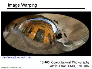
1. Computer Graphics Image warping and morphing

2. Image warping with slides by Richard Szeliski, Steve Seitz, Tom Funkhouser and Alexei Efros

3. B A Image formation

4. Sampling and quantization (179, 161, 153)

5. What is an image • We can think of an image as a function, f: R2R: • f(x, y) gives the intensity at position (x, y) • defined over a rectangle, with a finite range: • f: [a,b]x[c,d]  [0,1] • A color image f x y

6. A digital image • We usually operate on digital (discrete)images: • Sample the 2D space on a regular grid • Quantize each sample (round to nearest integer) • If our samples are D apart, we can write this as: f[i ,j] = Quantize{ f(i D, j D) } • The image can now be represented as a matrix of integer values

7. f f g h h x x x g x Image warping image filtering: change range of image g(x) = h(f(x)) h(y)=0.5y+0.5 image warping: change domain of image g(x) = f(h(x)) h(y)=2y

8. h h Image warping image filtering: change range of image f(x) = h(g(x)) h(y)=0.5y+0.5 f g image warping: change domain of image f(x) = g(h(x)) h([x,y])=[x,y/2] f g

9. Parametric (global) warping Examples of parametric warps: aspect translation rotation perspective cylindrical affine

10. T Parametric (global) warping • Transformation T is a coordinate-changing machine: p’ = T(p) • What does it mean that T is global? • Is the same for any point p • can be described by just a few numbers (parameters) • Represent T as a matrix: p’ = M*p p = (x,y) p’ = (x’,y’)

11. Scaling • Scaling a coordinate means multiplying each of its components by a scalar • Uniform scaling means this scalar is the same for all components: g f 2

12. x  2,y  0.5 Scaling • Non-uniform scaling: different scalars per component:

13. All 2D Linear Transformations • Linear transformations are combinations of … • Scale, • Rotation, • Shear, and • Mirror • Properties of linear transformations: • Origin maps to origin • Lines map to lines • Parallel lines remain parallel • Ratios are preserved • Closed under composition

14. 2D Translation? 2x2 Matrices • What types of transformations can not be represented with a 2x2 matrix? NO! Only linear 2D transformations can be represented with a 2x2 matrix

15. Translation • Example of translation Homogeneous Coordinates tx = 2ty= 1

16. Affine Transformations • Affine transformations are combinations of … • Linear transformations, and • Translations • Properties of affine transformations: • Origin does not necessarily map to origin • Lines map to lines • Parallel lines remain parallel • Ratios are preserved • Closed under composition • Models change of basis

17. Projective Transformations • Projective transformations … • Affine transformations, and • Projective warps • Properties of projective transformations: • Origin does not necessarily map to origin • Lines map to lines • Parallel lines do not necessarily remain parallel • Ratios are not preserved • Closed under composition • Models change of basis

18. Image warping • Given a coordinate transform x’= T(x) and a source image I(x), how do we compute a transformed image I’(x’)=I(T(x))? T(x) x x’ I(x) I’(x’)

19. T(x) Forward warping • Send each pixel I(x) to its corresponding location x’=T(x) in I’(x’) x x’ I(x) I’(x’)

20. Forward warping fwarp(I, I’, T) { for (y=0; y<I.height; y++) for (x=0; x<I.width; x++) { (x’,y’)=T(x,y); I’(x’,y’)=I(x,y); } } I I’ T x x’

21. Forward warping • Send each pixel I(x) to its corresponding location x’=T(x) in I’(x’) • What if pixel lands “between” two pixels? • Will be there holes? • Answer: add “contribution” to several pixels, normalize later (splatting) h(x) x x’ f(x) g(x’)

22. Forward warping fwarp(I, I’, T) { for (y=0; y<I.height; y++) for (x=0; x<I.width; x++) { (x’,y’)=T(x,y); Splatting(I’,x’,y’,I(x,y),kernel); } } I I’ T x x’

23. T-1(x’) Inverse warping • Get each pixel I’(x’) from its corresponding location x=T-1(x’) in I(x) x x’ I(x) I’(x’)

24. Inverse warping iwarp(I, I’, T) { for (y’=0; y’<I’.height; y’++) for (x’=0; x’<I’.width; x’++) { (x,y)=T-1(x’,y’); I’(x’,y’)=I(x,y); } } T-1 I I’ x x’

25. Inverse warping • Get each pixel I’(x’) from its corresponding location x=T-1(x’) in I(x) • What if pixel comes from “between” two pixels? • Answer: resample color value from interpolated (prefiltered) source image x x’ f(x) g(x’)

26. Inverse warping iwarp(I, I’, T) { for (y=0; y<I’.height; y++) for (x=0; x<I’.width; x++) { (x,y)=T-1(x’,y’); I’(x’,y’)=Reconstruct(I,x,y,kernel); } } T-1 I I’ x x’

27. Reconstruction • Computed weighted sum of pixel neighborhood; output is weighted average of input, where weights are normalized values of filter kernel k color=0; weights=0; for all q’s dist < width d = dist(p, q); w = kernel(d); color += w*q.color; weights += w; p.Color = color/weights; p width d q

28. Reconstruction (interpolation) • Possible reconstruction filters (kernels): • nearest neighbor • bilinear • bicubic • sinc (optimal reconstruction)

29. Bilinear interpolation • A simple method for resampling images

30. Non-parametric image warping • Specify a more detailed warp function • Splines, meshes, optical flow (per-pixel motion)

31. P’ Non-parametric image warping • Mappings implied by correspondences • Inverse warping ?

32. Barycentric coordinate P’ P Non-parametric image warping

33. Barycentric coordinates

34. Barycentric coordinate Non-parametric image warping

35. radial basis function Non-parametric image warping Gaussian thin plate spline

36. Demo • http://www.colonize.com/warp/warp04-2.php • Warping is a useful operation for mosaics, video matching, view interpolation and so on.

37. Image morphing

38. Cross dissolving is a common transition between cuts, but it is not good for morphing because of the ghosting effects. image #2 image #1 dissolving Image morphing • The goal is to synthesize a fluid transformation from one image to another.

39. Artifacts of cross-dissolving http://www.salavon.com/

40. Image morphing • Why ghosting? • Morphing = warping + cross-dissolving shape (geometric) color (photometric)

41. cross-dissolving warp warp morphing Image morphing image #1 image #2

42. Morphing sequence

43. Face averaging by morphing average faces

44. Image morphing create a morphing sequence: for each time t • Create an intermediate warping field (by interpolation) • Warp both images towards it • Cross-dissolve the colors in the newly warped images t=0 t=0.33 t=1

45. Warp specification (mesh warping) • How can we specify the warp? 1. Specify corresponding spline control points interpolate to a complete warping function easy to implement, but less expressive

46. Warp specification • How can we specify the warp 2. Specify corresponding points • interpolate to a complete warping function

47. Solution: convert to mesh warping • Define a triangular mesh over the points • Same mesh in both images! • Now we have triangle-to-triangle correspondences • Warp each triangle separately from source to destination • How do we warp a triangle? • 3 points = affine warp! • Just like texture mapping

48. Warp specification (field warping) • How can we specify the warp? • Specify corresponding vectors • interpolate to a complete warping function • The Beier & Neely Algorithm

49. Beier&Neely (SIGGRAPH 1992) • Single line-pair PQ to P’Q’:

50. Algorithm (single line-pair) • For each X in the destination image: • Find the corresponding u,v • Find X’ in the source image for that u,v • destinationImage(X) = sourceImage(X’) • Examples: Affine transformation