Download
1 / 27
270 likes | 510 Views
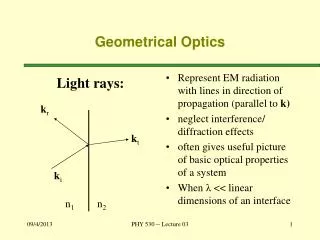
k r. k t. k i. n 1. n 2. Geometrical Optics. Represent EM radiation with lines in direction of propagation (parallel to k) neglect interference/ diffraction effects often gives useful picture of basic optical properties of a system When λ << linear dimensions of an interface.

E N D
kr kt ki n1 n2 Geometrical Optics • Represent EM radiation with lines in direction of propagation (parallel to k) • neglect interference/ diffraction effects • often gives useful picture of basic optical properties of a system • When λ << linear dimensions of an interface Light rays: PHY 530 -- Lecture 03
li lo R V P S n2 n1 q p Image Formation Imagine a spherical interface between two indices of refraction: C Optical axis PHY 530 -- Lecture 03
Definitions • S = point source of EM radiation • V = vertex of lens • P = image point (where rays/ spherical wavefronts converge) • p = “object distance” • q = “image distance” • R = radius of spherical interface • Assume n2 > n1 PHY 530 -- Lecture 03
Distance Conventions (Lenses) • For objects drawn on the left of the first vertex: • p: positive (object real) if to the left of V, negative if to the right (object virtual). • q: negative (image virtual) if to the left of V, positive if to the right (image real). • R: positive if C is to the right of V, negative if to the left. PHY 530 -- Lecture 03
Approximation To understand what is going on, let’s imagine that we Only care about rays traveling close to the optical axis. This means we will only deal with small angles. Try it! (q in radians) lp h q p PHY 530 -- Lecture 03
Image Formation f f1 f f2 lp h R lq f1 f V f2 x C I O n2 n1 q p PHY 530 -- Lecture 03
Now apply Snell’s Law Small angle approximation: Substitute for the angles: Small angle approximation in reverse: PHY 530 -- Lecture 03
Keep going… Looking at the picture: But x is a small number, so… PHY 530 -- Lecture 03
Finally… Rearranging, Or in other words, THIS DOES NOT DEPEND ON h, f1, or f2 !!! All rays close to the optical axis focus to the same point! PHY 530 -- Lecture 03
Implications... Choose P at infinity: “first focal length” = “object focal length” S V fo PHY 530 -- Lecture 03
More Implications... Choose S at infinity: “second focal length” = “image focal length” P V fi PHY 530 -- Lecture 03
li lo R1 R2 V2 V1 P S nl nm nm q p What is a Lens, Anyway? Two spherical surfaces: (assume nl>nm) PHY 530 -- Lecture 03
li lo R1 V2 V1 P P’ S nl nm nm q1 p Well, Consider the First Surface In the absence of the second surface, rays would converge at P’: PHY 530 -- Lecture 03
We Know the Solution! (*) Now, see figure on next slide. Can see that (Remember sign conventions! p2 is to the right of V2.) PHY 530 -- Lecture 03
Second Surface li lo R2 V2 V1 nm P P’ S nl nm q d p2 p q1 PHY 530 -- Lecture 03
We know the solution here too! Or, substituting for p2: (**) PHY 530 -- Lecture 03
Add two equations Adding (*) (slide 14) and (**) (slide 16), we have Now rearrange: PHY 530 -- Lecture 03
Thin Lens Approximation In the limit (lens thickness negligible compared with p, q) where PHY 530 -- Lecture 03
P S V1=V2 p q Thin lenses (2) In the thin lens approximation, V1, V2 coalesce into the same point. PHY 530 -- Lecture 03
Focal Lengths Note that, since the equation on slide 18) is symmetric in p and q, the image and object focal lengths are equal. S fo P fi Lensmaker’s Equation PHY 530 -- Lecture 03
P S V1=V2 p q Gaussian Lens Equation Gaussian form of the lens maker’s equation PHY 530 -- Lecture 03
L1 L2 P S Thin Lens Combinations d Similar to the two surface case, we will handle this in two pieces... PHY 530 -- Lecture 03
First Lens L1 L2 P P’ S q1 p In the absence of L2, image will form at P’, use Gaussian lens equation: PHY 530 -- Lecture 03
Second Lens L1 L2 P P’ S q d p2 q1 Real image Virtual image PHY 530 -- Lecture 03
Now the math... Okay, so lens 2 gives us Now, substitute for p2 Then substitute for q1. PHY 530 -- Lecture 03
Finally... Can show in the limit . (Lenses in contact.) In other words, the effective focal length of the combination is PHY 530 -- Lecture 03
N Thin Lenses in Contact One can keep going with the derivation to show that PHY 530 -- Lecture 03