Download
1 / 32
320 likes | 498 Views
Esci 203, Earth Structure and Deformation Using GPS for tectonic studies. John Townend EQC Fellow in Seismic Studies john.townend@vuw.ac.nz. Overview. A brief review of the last lecture Trilateration Measuring the distance to a satellite using pseudo-random code measurements

E N D
Esci 203, Earth Structure and DeformationUsing GPS for tectonic studies John Townend EQC Fellow in Seismic Studies john.townend@vuw.ac.nz
Overview • A brief review of the last lecture • Trilateration • Measuring the distance to a satellite using pseudo-random code measurements • Sources of error • Overcoming/reducing location errors • Using GPS to measure tectonic phenomena
The continuous GPS network Network status as of 7 May 2012
SV1 SV2 SV3 SV4 Trilateration • The receiver computes the distance (“pseudo-range”) to at least four satellites to calculate its position • This is “point positioning” and is like locating an earthquake in reverse (one receiver and many sources rather than one source and many receivers) distance = travel time speed of light
Pseudo-random codes • The signal emitted by each satellite is unique and extremely complex (“pseudo-random”) • The receiver generates the same signal, and compares it with what it receives from the satellite to determine the travel time Receiver signal t Satellite signal
Using phase measurements Observed phase difference Clock error We can measure the fractional phase difference between the satellite and receiver carrier signals, but unless we know the integer ambiguity we can’t estimate the pseudorange What we want Integer ambiguity ?
Sources of error • Ionospheric/tropospheric delays • Multi-pathing • Receiver clock errors • Ephemeris errors • Constellation geometry and weather • Intentional signal degradation: • “selective availability”, which limits accuracy to ~6–12 m
Ionospheric effects • The ionosphere is an ionised layer at ~100–1000+ km, which affects EM signal propagation • Frequency-dependent: n ~1/f2 • Ionospheric effects on pseudorange and phase measurements are opposite in sign • Using a dual-frequency receiver, the effects of the ionosphere can be estimated and accounted for One person’s noise is another person’s signal…
Tropospheric effects • This is the lowest, non-ionised portion of the atmosphere, and the effect on EM signal propagation arises from variations in temperature, pressure, humidity • The effects are frequency-independent, but a function of elevation (angle from the horizon) and tropospheric water content • The frequency-independence means that the troposphere’s effects have to be modelled
Multi-pathing actual signal path presumed signal path R It’s best to avoid buildings/trees etc.
presumed orbit and position actual orbit and position Ephemeris errors • The satellite’s orbit is specified by six ephemeris parameters at a reference epoch, and nine parameters describing the orbit’s evolution with time • The ground stations predict and send to the satellite the parameters that it broadcasts to receivers for use in real-time • “Precise ephemerides” are calculated over several weeks
Differential GPS (“dGPS”) • Reference stations broadcast corrections to the satellites’ signals; typical dGPS accuracy is ~1–5 m Satellite GPS signal GPS signal dGPS correction signal Mobile receiver Reference station
More complicated processing SVB SVA rA2(t2) rA2(t1) rB2(t2) rB2(t1) rA1(t1) rA1(t2) rB1(t2) rB1(t1) R1 R2
General strategy • Single differencing (2 receivers, 1 satellite) removes errors common to the satellite • Double differencing (2 receivers, 2 satellites) next removes errors common to the receivers • Triple differencing (2 receivers, 2 satellites, 2 epochs) removes integer ambiguities, but reduces geometric constraints on the solutions
NZ on the move Animation kindly provided by John Beavan, GNS Science
Vigny et al., Nature 2005 Modelling the Sumatra earthquake Model of a single fault segment Model of two fault segments
Subarya et al., Nature 2005 GPS vs. seismology
Vigny et al., Nature 2005 Postseismic slip
Fig. 1 Map of central and northern Honshu, Japan. M Simons et al. Science 2011;332:1421-1425 Published by AAAS
Fig. 3 Inferred distribution of subsurface fault slip (color and black contours with a contour interval of 8 m). M Simons et al. Science 2011;332:1421-1425 Published by AAAS
Fig. 1 Horizontal (A) and vertical (B) coseismic displacements at the sea-floor reference points, associated with the 2011 Tohoku-Oki earthquake. M Sato et al. Science 2011;332:1395-1395 Published by AAAS
Fig. 2 (A) Observed (green) and predicted (white) deep ocean tsunami records of the Tohoku-Oki earthquake. M Simons et al. Science 2011;332:1421-1425 Published by AAAS
Not all slip is quick Delahaye et al., 2009
Slow slip summary After Douglas et al. (2005), Wallace and Beavan (2006) CGPS Broadband • Gisborne ~20 cm slip, 14 km depth, ~12 day • Hawke’s Bay ~5-10 cm slip, 12 km depth, ~7 day • Manawatu 30 cm slip, 25-30 km depth, 1.5 yr • Kapiti 50 cm slip, 30-35 km depth, ~1 yr • Cook Strait, ~1 yr? (J. Beavan, pers. comms.) 1 2 3 4 5
Summary • Points to revise • Strategies for accurately measuring positions and reducing uncertainties • Examples of how GPS data can be used • Extra material online • http://www.unavco.org/edu_outreach/data.html (easily accessible data and exercises)
Reading material • Van der Pluijm and Marshak • Section 14.9 • Fowler (2005) • Sections 2.1 and 2.2 • Mussett and Khan • Section 20.5