Download

1 / 18
180 likes | 201 Views
Explore the characteristics and applications of Uniform and Normal distributions in probability theory. Learn how to calculate probabilities and solve real-world problems using these distributions.

E N D
Lecture 1Uniform and Normal Distributions Walpole Chapter 6 Continuous Probability Distributions
Continuous Probability Distributions • Many continuous probability distributions, including: • Uniform • Normal • Gamma • Exponential • Chi-Squared • Lognormal • Weibull Weibull PDF Source: www.itl.nist.gov EGR 252 JMB 2019
Uniform Distribution • Simplest continuous probability distribution – characterized by the interval endpoints, A and B. A ≤ x ≤ B = 0 elsewhere • Mean and variance: and EGR 252 JMB 2019
Example: Uniform Distribution A circuit board failure causes a shutdown of a computing system until a new board is delivered. The delivery time X is uniformly distributed between 1 and 5 days. What is the probability that it will take 2 or more days for the circuit board to be delivered? EGR 252 JMB 2019
In Class Examples • 6.3 EGR 252 JMB 2019
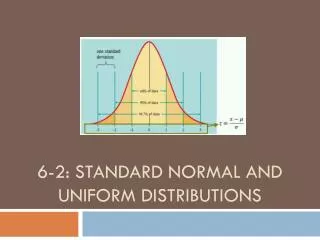
Normal Distribution • The “bell-shaped curve” • Also called the Gaussian distribution • The most widely used distribution in statistical analysis • forms the basis for most of the parametric tests we’ll perform later in this course. • describes or approximates most phenomena in nature, industry, or research • Random variables (X) following this distribution are called normal random variables. • the parameters of the normal distribution are μand σ(sometimes μand σ2.) EGR 252 JMB 2019
(μ = 5, σ = 1.5) Normal Distribution • The density function of the normal random variable X, with mean μ and variance σ2, is all x. EGR 252 JMB 2019
Standard Normal RV … • Note: the probability of X taking on any value between x1 and x2 is given by: • To ease calculations, we define a normal random variable where Z is normally distributed with μ = 0 and σ2= 1 EGR 252 JMB 2019
Standard Normal Distribution • Table A.3 Pages 735-736: “Areas under the Normal Curve” EGR 252 JMB 2019
Examples • P(Z ≤ 1) = • P(Z ≥ -1) = • P(-0.45 ≤ Z ≤ 0.36) = EGR 252 JMB 2019
Name:________________________ • Use Table A.3 to determine (draw the picture!) 1. P(Z≤ 0.8) = 2. P(Z≥ 1.96) = 3. P(-0.25 ≤ Z≤ 0.15) = 4. P(Z ≤ -2.0 orZ≥ 2.0) = EGR 252 JMB 2019
Applications of the Normal Distribution • A certain machine makes electrical resistors having a mean resistance of 40 ohms and a standard deviation of 2 ohms. What percentage of the resistors will have a resistance less than 44 ohms? • Solution: Xis normally distributed with μ = 40 and σ= 2 and x = 44 P(X<44) = P(Z< +2.0) = 0.9772 Therefore, we conclude that 97.72% will have a resistance less than 44 ohms. What percentage will have a resistance greater than 44 ohms? EGR 252 JMB 2019
The Normal Distribution “In Reverse” • Example: Given a normal distribution with μ = 40 and σ = 6, find the value of X for which 45% of the area under the normal curve is to the left of X. Step 1 If P(Z < z) = 0.45, z = _______ (from Table A.3) Why is z negative? Step 2 X = _________ 45% EGR 252 JMB 2019
In-Class Exercise 6.14 The finished inside diameter of a piston ring is normally distributed with a mean of 10 centimeters and a standard deviation of 0.03 centimeter. • What proportion of rings will have inside diametersexceeding 10.075 centimeters? (b) What is the probability that a piston ring will havean inside diameter between 9.97 and 10.03 centimeters? (c) Below what value of inside diameter will 15% of thepiston rings fall?of 0.03 centimeter. EGR 252 JMB 2019
In-Class Exercise 6.14 Solution • What proportion of rings will have inside diametersexceeding 10.075 centimeters? Draw the picture!!!!! How do we know the vertical line is to the right of center? (b) What is the probability that a piston ring will havean inside diameter between 9.97 and 10.03 centimeters? EGR 252 JMB 2019
In-Class Exercise 6.14 Solution (b) What is the probability that a piston ring will have an inside diameter between 9.97 and 10.03 centimeters? Can you draw the graphic using Z values???? Can you draw the graphic using x values???? (c) Below what value of inside diameter will 15% of the piston rings fall? of 0.03 centimeter. EGR 252 JMB 2019
In-Class Exercise Based on 6.17 (page 187) The average life of a certain type of small motor is 10 years with a standard deviation of 2 years. The manufacturer will give a free replacement for all motors that fail while under guarantee. If she is willing to replace only 3% of the motors, how long a guarantee should be offered? Assume that the lifetime of a motor follows a normal distribution. EGR 252 JMB 2019
In-Class Exercise Based on 6.17 The average life of a certain type of small motor is 10 years with a standard deviation of 2 years. The manufacturer will give a free replacement for all motors that fail while under guarantee. If she is willing to replace only 3% of the motors that fail, how long a guarantee should be offered? Assume that the lifetime of a motor follows a normal distribution. Step 1: Find the value of Z such that 3% of the area under the curve is to the left. Step 2: Use Z , µ, σvalues to solve for X. 97% Step 2 Solve for X X = (2 * -1.88) + 10 = 6.24 A vertical line at x = 6.24 will have 3% of the area under the curve to the left. 3% Z = -1.88 Step 1 A z-value of -1.88 corresponds to 3% of the area under the curve EGR 252 JMB 2019