Download
1 / 70
710 likes | 959 Views
Suffix Trees and their applications. Amit Metodi and Tali Weinberger. Seminar 2012/1. Outline. Introduction to Suffix Trees Trie and Compressed Trie Suffix Tree Trivial Construction Algorithm O(N^2) Exact string matching Generalized suffix tree Applications. Trie.

E N D
Suffix Treesand their applications AmitMetodi and Tali Weinberger Seminar 2012/1
Outline • Introduction to Suffix Trees • Trie and Compressed Trie • Suffix Tree • Trivial Construction Algorithm O(N^2) • Exact string matching • Generalized suffix tree • Applications
Trie • A tree representing a set of strings.(Assume no string is a prefix of another) • Each edge is labeled by a letter. • No two edges outgoing from thesame node are labeled the same. • Each string corresponds to a leaf. c a b d e b e f e g f “aeef “ { “aeef “ , “ad“ , “bbfe “ , “bbfg “ , “c “ }
Compressed Trie • Compress unary nodes, label edges by strings. • All internal non-root nodes are branching, there can be at most n−1 such nodes, and n+(n−1)+1= 2n nodes in total(n leaves, n−1 internal nodes, 1 root). c c a a b d d e b eef bbf e f e g e g f { “aeef “ , “ad“ , “bbfe “ , “bbfg “ , “c “ }
Suffix Tree • A suffix tree of string S[1..n] is a compressed trie of all suffixes of S. • Denote S[i..n] bySi • S = “x a b x a c” • 1 2 3 4 5 6 • { • S6= c • S5= ac • S4= xac • S3= bxac • S2=abxac • S1=xabxac • } a c xa 6 c Does a suffix tree always exist ? 5 bxac c bxac 4 bxac 3 2 1
Suffix Tree • S = “x a b x a” • 1 2 3 4 5 • { • S5= a • S4= xa • S3= bxa • S2=abxa • S1=xabxa • } a xa 5 4 bxa bxa bxa 3 2 1 The fourth suffix xa or the fifth suffix a won’t be represented by a leaf node.
Suffix Tree • Solution: insert a special terminal character at the end such as $. • Then, xa$ will not be a prefix of the suffix xabxa$. • S = “x a b x a $” • 1 2 3 4 5 6 • { • S6= $ • S5= a$ • S4= xa$ • S3= bxa$ • S2=abxa$ • S1=xabxa$ • } a $ xa 6 $ 5 bxa$ $ bxa$ 4 bxa$ 3 2 1
Trivial algorithm to build Suffix tree Build suffix tree S=xaxac (S’=xaxac$) • Put the largest suffix xaxac$ • Put the suffix axac$ • Put the suffix xac$ a x x a a x c a c $ $
Trivial algorithm to build Suffix tree Build suffix tree S=xaxac (S’=xaxac$) • Put the largest suffix xaxac$ • Put the suffix axac$ • Put the suffix xac$ • Put the suffix ac$ x a a x a c x c a $ $ c $
Trivial algorithm to build Suffix tree Build suffix tree S=xaxac (S’=xaxac$) • Put the largest suffix xaxac$ • Put the suffix axac$ • Put the suffix xac$ • Put the suffix ac$ • Put the suffix c$ • Put the smallest suffix $ • Label each leaf withthe starting point. c $ $ x a 5 a 6 c $ x c x a a $ 4 c c $ 3 $ 2 1
Complexity – Run Time • We need O(n-i+1) time for the ith suffix. Therefore the total running time is: • Ukkonen in 1995 provided the first online-construction of suffix trees with the running time that matched the then fastest algorithms. These algorithms are all linear-time for a constant-size alphabet, and have worst-case running time of O(nlogn) in general. • Martin Farach in 1997 gave the first suffix tree construction algorithm that is optimal for all alphabets O(n)
Complexity - Space • Will also take O(n2) if we would store every suffix in the tree separately. • Note that, we should not store the actual substringsS[i ... j] of S in the edges, but only their start and end indices (i, j). • Nevertheless we keep thinking of the edge labels as substrings of S. • This will reduce the space complexity to O(n)
Exact string matching • Given S and P strings where |S|=n and |P|=m. Find all occurrences of P in S. • Naïve algorithm = O(n*m) S= 2 5 P=
Exact string matching • Given S and P strings where |S|=n and |P|=m. Find all occurrences of P in S. Using suffix tree: 1. Build suffix tree O(n) 2. Try to match P on a path. Three cases: a. No match → P does not occur in T. b. The match of P ends in a node u. Set x = u. c. The match ends inside an edge (v,w). Set x=w. O(m) 3. All leaves below x represent occurrences of P. O(k) (where k = number of occurrences of P in S) Total time: O(n+m+k) ~= O(n) p s i $ p s p s i 11 i $ mississippi$ 8 s p s p i i p p $ i $ 5 1 2
Generalized suffix tree • Given a set of strings T a generalized suffix tree of T is a compressed trie of all suffixes of S T. • To make these suffixes prefix-free we add a special char at the end of S. • To associate each suffix with a unique string in T, add a different special char to each S T.
Generalized suffix tree • Let S1=ababand S2=aab here is a generalized suffix tree for S1 and S2 $ # a b { $ # b$ b# ab$ ab# bab$ aab# abab$ } 4 5 # b a a $ 3 b b # $ 4 a # 1 2 b $ $ 2 3 1
Applications of suffix trees • Longest Common Substring • DNA Contamination Problem • Maximal Repetitive Structures • Longest common extension • Finding maximal palindromes • The k-mismatch problem
Longest Common Substring • Given strings A and B find the longest substring common to both strings. • String A= lambada • String B=abady • Longest Common Substring = bad Donald E. Knuth conjectured in 1970 that It is impossible to solve this Longest Common Substring problem in O(|A|+|B|) time.
A # B $ LCSubstring - Idea • Construct a suffix tree T for A#B$, where # and $ are two characters not in A and B. • There are exactly |A|+|B|+2 leaves in T, each leaf corresponds to a suffix of A#B$. • A-leaf: with label in {1, 2, …, |A|} • corresponds to an A-suffix. • B-leaf: with label in {|A|+2, …,|A|+|B|+1} • corresponds to a B-suffix. B-suffix A-suffix
LCSubstring - Observation • Let v be an arbitrary position of T (i.e., v is not necessarily a node of T.) • v has a descendant A-leaf if and only if v corresponds to a prefix of an A-suffix of A#B$. • v has a descendant B-leaf if and only if v corresponds to a prefix of a B-suffix of A#B$. root v
A # B $ LCSubstring - Lemma • Let v be a position of T.v has descendant A-leaf and B-leafif and only if v corresponds to a common substring ofA and B. root v v v B-suffix v v A-suffix
LCSubstring – Algorithm • Construct a suffix tree T for A#B$. O(|A|+|B|) • Marking the colors of each node, including each leaf and each internal nodes. O(|A|+|B|) • Computing the depths of all nodes. O(|A|+|B|) • Find a deepest internal node with both colors. O(|A|+|B|) • Output the string corresponding to the deepest internal node v such that the subtree of T rooted at vcontains both A-leaf and B-leaf. • Time:O(|A|+|B|) • Space: O(|A|+|B|) Single DFS Space can be reduced to O(|A|)
LCSubstring - Example • Let A=aabcyand B=abab, here is a generalized suffix tree for Aand B. # y * # * { $#* b$y#* ab$cy#* bab$bcy#* abab$abcy#* aabcy#* } 6 $ c 5 y a # * b 11 4 c y # * b a b a $ 3 c b y $ c # 10 a y * b $ 8 # $ * 1 7 9 2
LCSubstring - Example • Let A=aabcyand B=abab, here is a generalized suffix tree for Aand B. # y # { $# b$y# ab$cy# bab$bcy# abab$abcy# aabcy# } 0 6 $ c 5 y a # b 5 4 1 c y # 1 b a b a $ 3 c b y 2 $ c # 4 a y b $ 2 # $ 1 1 3 2
DNA Contamination Problem DNA contamination: During laboratory processes, unwanted DNA insertedinto the DNA of interest. Contamination sources: Human, bacteria,… DNA from Dinosaur bone: More similar to human DNA than to bird and crockodilian DNA
DNA Contamination Problem S: DNA of interest P: DNA of possible contamination source If S and P share a common substring longer than l, then S has been contaminated by P. To find all common substrings of S and P that are longer than l . In general, P is set of DNA that are potential contamination sources.
Applications of suffix trees • Longest Common Substring • DNA Contamination Problem • Maximal Repetitive Structures • Longest common extension • Finding maximal palindromes • The k-mismatch problem
Maximal Pair • A maximal pair in string S:A pair of identical substrings a and b in S s.t. the characters to the immediate left and right of a is different from the characters to the immediate left and right of b, respectively. • That is, Extending a and b in either direction would destroy the equality of the two strings. • Example: S = xabcyiiizabcqabcyrxar
Maximal Pair (continued) • Overlap is allowed:S = cxxaxxaxxbcxxaxxaaxxaxxb • To allow a prefix or suffix of S to be part of a maximal pair:S #S$ (#,$ don’t appear in S).Example: #abcxabc$
Maximal Repeat • A maximal repeat in string S: A substring of S that occurs in a maximal pair in S. • Example: S = xabcyiiizabcqabcyrxar maximal repeats: abc, abcy, ...
Finding All Maximal RepeatsIn Linear Time • Given: String S of length n. • Goal: Find all maximal repeats in O(n) time. • Lemma: Let T be a suffix tree for S.If string a is a maximal repeat in S,then a is the path-label of an internal node v in T.
Proof – by def. of maximal repeat S = xabcyiiizabcqabcyrxar root a a b c v y q • A maximal repeat in string S: A substring of S that occurs in a maximal pair in S.
Observation • T has at most n internal nodes. • Why? Since T has n leaves (one for each index), and each internal node other than the root must have at least two children, T can have at most n internal nodes.
Conclusion • There can be at most n maximal repeats in any string of length n. • Proof: by the lemma, since T has at most n internal nodes.
Which internal nodes correspond to maximal repeats? • The left character of leaf i in T is S(i-1). • Node v of T is called left diverse if at least 2 leaves in v’s subtree have different left characters. • A leaf can’t be left diverse. • Left diversity propagates upward.
Example: S = #xabxa$1 2 3 4 5 6 left diverse maximal repeat xa a bxa$ $ 3 6 a a bxa$ bxa$ $ $ 5 2 4 5 2 4 1 x x b #
Theorem The string a labeling the path to an internal node v of T is a maximal repeat v is left diverse.
Proof of • Suppose a is a maximal repeat • It participates in a maximal pair • It has at least two occurrences with distinct left characters: xa, ya, xy • Let i and j be the two starting positions of a. Then leaves i and j are in v’s subtree and have different left characters x,y. • v is left diverse.
Proof of • Suppose v is left diverse there are substrings xap and yaq in S, xy. • If pq a’s occurrences in xap and yaq form a maximal pair a is a maximal repeat. • If p=q since v is a branching node, there is a substring zar in S, rp.If zx It forms a maximal pair with xap.If zy It forms a maximal pair with yap.In either case, a is a maximal repeat. These cases cover all the cases, since xy.
Proof of (continued) root root Case 1: Case 2: a a v v r... p... p… q… left char x left char y left char z left char x left char y
Compact Representation • Node v in T is a frontier node if: • v is left diverse. • none of v’s children are left diverse. • Each node at or above the frontier is left diverse. • The subtree of T from the root down to the frontier nodes is the compact representation of the set of all maximal repeats of S. • Representation in O(n) though total length of all maximal repeats may be larger.
Linear time algorithm • Build suffix tree T. • Find all left diverse nodes in linear time. • Delete all nodes that aren’t left diverse, to achieve the compact representation.
finding all left diverse nodes in linear time • Traverse T bottom-up, recording for each node: • either that it is left diverse • or the left character common to all leaves in its subtree. • For each leaf: record its left character. • For each internal node v: • If any child is left diverse v is left diverse. • Else If all children have a common character x record x for v. • Else record that v is left diverse.
Time Analysis • Suffix tree construction O(n). • Bottom-up traversal O(n). • Total O(n).
Applications of suffix trees • Longest Common Substring • DNA Contamination Problem • Maximal Repetitive Structures • Longest common extension • Finding maximal palindromes • The k-mismatch problem
Longest common extension Longest common extension: a bridge to inexact matching
Longest common extension problem Preprocess strings S1 and S2s.t. the following queries can be computed in O(1) time each: • Given index pair (i,j), find the length of the longest substring of S1 starting at position i that matches a substring of S2 starting at position j. S1: ... abcdzzz ... S2: ... abcdefg ... j i
Lowest common ancestors A lot more can be gained from a suffix tree if we preprocess it so that we can answer LCA queries on it
Why to find LCA? For two suffixes of S, we can compute their Longest Common Prefixby finding the LCA of the corresponding leaves in the suffix tree. LCP(ippi$,issippi$)= i $ p s mississippi$ 12 si i $ 1 i$ ppi$ pi$ ssi$ 8 9 11 10 ssippi$ ssippi$ ppi$ ppi$ ppi$ ssippi$ 2 5 3 7 4 6