Download
1 / 30
300 likes | 403 Views
Augmenting Suffix Trees, with Applications. Yossi Matias, S. Muthukrishnan, Suleyman Cenk Sahinalp, Jacob Ziv. Presented by Genady Garber. Abstract. Theory of string algorithms play a fundamental role in Information retrieval Data compression

E N D
Augmenting Suffix Trees, with Applications Yossi Matias, S. Muthukrishnan, Suleyman Cenk Sahinalp, Jacob Ziv Presented by Genady Garber
Abstract • Theory of string algorithms play a fundamental role in • Information retrieval • Data compression • This work consider one algorithmic problem from each area. • The algorithms rely on augmenting the suffix tree (adding extra edges, resulting DAGs) • The algorithm construct these “suffix DAGs” and manipulate them to solve the problems.
Introduction • This paper presents two algorithmic problems • Data Compression • Information Retrieval • All these algorithms rely on the suffix tree data structure • ST with suitably simple augmentations are very useful in string processing applications • In described work the suffix tree was augmented with extra edges and additional information
Problems and Background • The Document Listing Problem • The HYZ Compression Problem
The Document Listing Problem • Given a set of documents T = {T1, . . . , Tk} • Given a query pattern P • The problem • To output a list of all documents containing P as a substring (the standard problem can be solved in time, proportional to number of occurrences of P in T. The goal is to solve the problem with a running time depending on the number of documents containing P) • To report the number of documents containing P(existing algorithm solves this problem in O(|P|) and is based on data structures for computing Lowest Common Ancestor) • May be used in “morbid “applications (discovering gene homologies)
The (a,b)-HYZ Compression Problem • Given a binary string T of length t • Need to replace disjoint blocks of size b with desirably shorter codewords(to allow future perfect decompression) Compression Algorithm • To compute the codeword cjfor block j we determine its context (the context of a block T[i : l] is the longest substring T[k : i - 1], k < i, of size at most a , T[k : l] occurs earlier in T) • The codeword cj is the ordered pair {g , l} where • g - length of the context of block j • l- rank of block jwithrespect to the context (according to some predetermined order - lexicographic, etc.) • Intuition: similar symbols in data appear in similar contexts
The (a,b)-HYZ Compression Problem (previous results) • Case ofb = O(1) and ais unbounded • Average length of a codeword is shown to approach the conditional entropy for the block, within additive term of c1logH(C) + c2 for constants c1and c2, provided that the input is generated by a limited order Markovian source. • Case ofb >= loglog t and a= O(log t) • This scheme also achieves the optimal compression (in terms of CO) • Applies for all ergodic sources
The problem state Consider a set of document strings T = {T1, T2, . . . Tk}, of sizes t1, t2, . . . , tk. The goal is to build a data structure, supporting the following queries on an on-line pattern P of size p: • list query (the list of documents containing P) • count query (the number of documents containing P) Theorem 1 Given T and P, there is a data structure which responds to a count query in O(p) time, and a list query in O(plogk + out) time, where out is the number of documents in T that contain P.
The Suffix-DAG Data Structure Proof Sketch • Build the suffix-DAG of documents T1, . . ., Tk, in O(t) = O(Stk), using O(t) space • The suffix-DAG of T, denoted by SD(T), contains the generalized suffix tree, GST(T), of the set T at its core. • A GST(T) is defined to be the compact trie of all the suffixes of each of the documents in T. • Each leaf node l in GST(T) is labeled with the list of documents which have a suffix represented by the path from the root to l. • The substring represented by a path from the root to any given node n denoted by P(n)
The Suffix-DAG Data Structure (cont) • The nodes of SD(T) are the nodes of GST(T) • The edges of SD(T) are of two types: • the skeleton edges of SD(T) are the edges of GST(T) • the supportive edges of SD(T) are defined as follows:for any nodes n1and n2 in SD(T) there is a pointer edge from n1to n2 if and only if: • n1 is an ancestor of n2 • among the suffix trees ST(T1), ST(T2), . . . , ST(Tk) there exists at least one , say ST(Ti), which has two nodes , n1 , I and n2 , I such that • P(n1) = P(n1 , i) ,P(n2) = P(n2 , i) • n1 , I is the parent ofn2 , I • such an edge is labeled with I for all relevant documents in Ti
The Suffix-DAG Data Structure (cont.2) • In order to respond to the count and list queries, one of the standard data structures that support least common ancestor (LCA) queries on SD(T) in O(1) time was built. • Also each internal node n of SD(T) contains • array that stores its supportive edges in pre-order fashion • number of documents which include P(n) as substring
ST(T3) ST(T2) ST(T1) a a a c b b b b a c b a c c a c c # b b # b b # # # b a a # # # # # # # Example • The independent suffix trees • T1: abcb ; T2: abca ; T3: abab
a c b b c a a # b c b a b # b # a b # a # # # # # # # 1 2 3 1 3 1,3 2 1 2 3 2 Example (cont.) • The generalized suffix tree of the set of documents {T1, T2, T3} SK(T)
a c b b c a a # b c b a b # b # a b # a # # # # # # # 1 2 3 1 3 1,3 2 1 2 3 2 Example (cont.2) • The suffix-DAG of the set of documents 2 SD(T) 1,3 2 1 1 3 1
a c b b c a a # b c b a b # b # a b # a # # # # # # # 1 2 3 1 3 1,3 2 1 2 3 2 Example (cont.3) • The suffix-DAG of the set of documents legend: skeleton edge SD(T) number of documents in the subtree and the pointer array 3 1,3,2,1,3,2,1 2,2 3 3 3,1,3,1 2 - 3,1 3 2 - - 2
Lemmas and Proofs • Lemma1 The suffix-DAG is sufficient to respond to the count queries in O(p) time, and to list queries in O(p log k + out) time • Proof Sketch • To respond to count queries do as follows: • with P, trace down GST(T) until the highest level node n is reached for which P is a prefix of P(n) • return the number of documents that contain P(n) as a substring • To respond to list queries do as follows • locate n in SD(T) (defined above) and traverse SD(T) backwards from n to the root • at each node u on the path determine all supportive edges out of u have their endpoints in the subtree rooted at n
Lemmas and Proofs (cont.) • Complexity of list queries • the key observation is that all corresponding edges will form a consecutive segment. • the segment may be identified with two binary searches (performing an LCA query, it takes O(1) time) • maximum size of the array of supportive edges in any node is at most k|S| , where |S| = O(1) ( size of alphabet), that means this procedure takes O(log k) at each node u • the output at all such segments may contain duplicate, but total size of the output is O(out|S|) = O(out), where out is the number of occurrences of P in t
Lemmas and Proofs (cont.2) • Lemma 2 The suffix-DAG of the document set T can be constructed in O(t) time and O(t) space • Proof Sketch • The construction of GST(T) with all suffix links and data structure are standard • To complete SD(T) it is necessary • to construct supportive edges • to build supportive edge array • to explain, how the number of documents that include P(n) is computed
Lemmas and Proofs (cont.3) • Proof Sketch (cont.) • the supportive edge with label i can be built by emulating constriction for ST(Ti) (for each node is ST(Ti), there is a corresponding node in SD(T) with the appropriate suffix link) • supporting edges building • if there is supportive edge between nodes n1 and n2 , then either there is SE between n1`( there is suffix link from ni to ni`) and n2`, or there exist one intermediate node to which there is a supportive edge from n1` (n2`). • The time to compute such nodes as length of string between nodes n1 and n2 • to compute the number of documents #(n), containing the substring of n we need: • the number of supportive edges from n to its descendants # • the number of supportive edges to n from its ancestors # (n) (n)
Lemmas and Proofs (cont.4) • Lemma 3 For any node n, #(n) = Sn` E children of n #(n`)+ • Proof • if a document Tiincludes the substring of more than one descendant of n, then there should exist a node in ST(Ti) whose substring is identical to that of n • for any two supportive edges from n to n1 and n2, the path from n to n1 and the path from n to n2do not have any common edges +
The Compression Algorithm • Compression scheme Ca,b terms • the input is a string T of size t • binary alphabet • The scheme • partition the T into contiguous substrings (blocks) of size b • replace each block by a corresponding codeword (function of context) • the context of a block T[i : j] is the longest substring T[k : i-1] for k < I, for which T[k :l] occurs earlier in T. • if context exceeds a it truncated for a rightmost characters • the codeword cj is ordered pair <g,l>, where • gis the context size • l is the lexicographic order of block jamongall possible substrings of size b immediately following earlier occurrences of context of block j
Compression Example • T = 010011010 • a = 2 , b = 1 • the context of block 9 is T[7 : 8] = 01 • the two substrings which follow earlier occurrences of this context are T[3] = 0 and T[6] = 1 • the lexicographic order of block 9 amount these substrings is 1
The Compression Algorithm(cont) • Theorem 2 There is an algorithm to implement the compression scheme Ca,bwhich runs in O(tb) time and requires O(tb) space, independent of a • Proof Building suffix tree we augment it as follows • for each node v we store an array of size b in which for each i = 1, . . ., b: • store the number of distinct paths rooted at v of precisely i characters minus the number of such distinct paths of precisely i-1 characters (the number may be negative)
The Compression Algorithm(cont.2) • Lemma 4 There is an algorithm to construct the augmented suffix tree of T in O(tb) time • Proof While inserting a new node into suffix tree, update the subtree information of the ancestors of v which are at most b characters higher than v • number of such ancestors is at most b • at most one of the b fields of information at any ancestor of v needs to be updated
The Compression Algorithm(cont.3) • Lemma 5 The augmented suffix tree is sufficient to compute the codeword for each block of input T in amortized O( ) • Proof Sketch • The computation of g can be performed by locating the node in the suffix tree which represents the longest prefix of the context (can be achieved by using the suffix links in amortized O(b) time) • The computation of l • traverse the path between v and w (v represents the longest prefix of the context of block j, w, the descendant of v, represents the longest prefix of the substring formed by concatenating of lock j and its context) • during traversal, compute size of the relevant subtrees that smaler/greater then the substring represented by this path
The Compression Algorithm(cont.4) • Theorem 3 There is an algorithm to implement the compression method Ca,bfor a = log t and b = log log t in O(t) time using O(t) space • Proof Sketch For any descendents wi of v which are b chars apart from v, the DataStructure enables to compute lexicographic order of the path between any wi and v, allowing easy computation of codeword of block of size brepresented by path between v and wi • The algorithm exploits the fact that the context size is bounded, and its seeks similarities between suffixes of the input up to a small size.
The Compression Algorithm(cont.5) • Lemma 6 The augmented limited suffix tree of input T is sufficient to compute the codeword for any input block j in O(b) time • Proof Sketch • Given a block j of the input • v represents its context • w (descendant of v) represents substring: context(j) + block(j) • b = loglogt => the maximum number of elements in the search data structure for v is = O(logt) • there is a simple data structure that maintains k elements and compute the rank of any given element in O(log k) time • the lexicographic order of node w in only O(log log t) = O(b) time may be computed (in future work).
The Compression Algorithm(cont.6) • Lemma 7 The augmented limited suffix tree of input T can be built and maintained in O(t) time • Proof Sketch • The depth of augmented limited suffix tree is bounded by log t => the total number of nodes in the tree is only O(t), allowing to adapt ST construction in O(t) time - without being penalized for building a suffix trie rather than the suffix tree. • Because of each node v is inserted to the search data structure of at most one of its ancestors, it is possible to construct and maintain the search data structure of all nodes in O(t) time, => the total number of elements maintained by all search data structures is O(t) • The insertion time of an element e to a search DS is O(1) • As the total number of of nodes to be inserted is the DS is bounded by O(t), it may be shown, that the total time for insertion of nodes in the search DS is O(t)
Results and conclusions Document listing problem • Processing kdocuments in linear time ( O(Siti) ) and space • Time to answer a query with pattern P is O(|P|logk + out) • The fastest known algoritm runs in time proportional to number of occurrences of the pattern in all documents.
Results and conclusions (cont.) (a,b )-HYZ compression problem • unbounded a, complexity O(tb) • gives linear time for b = O(1) • The only previously known algorithm, where for b = O(1), the author presents an O(ta) time algorithm, and for unbounded a this running time is O( ) • a = O(log t), b = loglogt, complexity O(t) • There is no any previously known algorithms