Download

1 / 54
540 likes | 740 Views
Compressed Suffix Arrays and Suffix Trees. Roberto Grossi, Jeffery Scott Vitter. Outline. Reminders Motivation Compression results Time & Space bounds Compressed Suffix Tree Compressed Suffix Array Proof of bounds. Reminder - Symbols. T = t 1 t 2 ... t n - 1 text of length n-1

E N D
Compressed Suffix Arrays and Suffix Trees Roberto Grossi, Jeffery Scott Vitter
Outline • Reminders • Motivation • Compression results • Time & Space bounds • Compressed Suffix Tree • Compressed Suffix Array • Proof of bounds
Reminder - Symbols • T = t1t2...tn-1 • text of length n-1 • eof symbol # at the nth position • T[i,n] is suffix i of text T • i=1,…,n
Reminder - Symbols • P= p1p2...pm • pattern of length m • 0<ε≤1
Reminder - Main Goal • Search string pattern P within text T • Support fast queries • Text T being fully scanned only once
Reminder – Suffix Trees • Leaf with value i represents suffix [i,n] • Build time • O(n) • Search time • O(m) • Structure space • O(n)
Reminder – Suffix Arrays Lexicographically ordered SA[i] = the starting position in T of the i-th suffix Σ={a,b} a<#<b T = bbba# 1 2 3 4 5 4 5 3 2 1 a# # ba# bba# bbba#
Reminder – Suffix Arrays • Build time • O(nlogn) • Search time • O(m+logn) • Structure space • O(n)
Motivation • So Far • Greedy in space • Fast searching • Need for space-efficient text indexing • Reduce both space and query time
Compressed Suffix Tree • Build time • O(n) • Search time • O(m/logn+(logn)ε) • Structure space • (ε-1+O(1))n
Compressed Suffix Tree • Build Suffix Array • Build Compressed Suffix Tree • Patricia Tries • Compress Suffix Array
CSA Basic Operations • Compress(T,SA) • Return succinct representation of SA • Retain T • Discard SA • Lookup(i) • Return SA[i] • Use compressed SA
CSA Primary measures • Compress • Preprocessing compressed SA • Space of compressed SA • lookup • Query time
Compressed Suffix Array • Build time • O(n) • Structure space • ½nloglogn + O(n) • lookup time • O(loglogn)
Suffix Arrays Optimization • Main idea • Decomposition scheme • Recursive structure of permutations
Decomposition Scheme • K levels, K=0,….,l • SA0 =SA (Original SA) • n 0=n • n = |T| • assumption - n is a power of 2 • n k=n/2k • SAk={1,2,…,nk)
SAk Succinct Representation • 4 main steps: • Produce bit vector Bk • Map Bk 0’s to 1’s • Compute 1’s for each prefix in Bk • Using function rankk(j) • ‘Pack’ SAk
T = bba# 3 0 4 1 2 1 1 0 Step #1: Produce bit vector Bk • |Bk| = nk • Bk[i]=1 if SAk[i] is even Bk[i]=0 if SAk[i] is odd SA0 Bo
T = bba# 2 3 0 4 2 1 2 3 1 3 1 0 Step #2 : Map Bk 0’s to 1’s • New Fuction Ψk(i), i=1,…,nk • Ψk(i)= • jSAk[i] is odd • and SAk[j]= SAk[i]+1 • i otherwise (SAk[i] is even) SA0 Bo Ψo
T = bba# 0 3 0 4 1 1 2 2 1 1 2 0 Step #3 : Compute 1’s for Bk • Recall fuction rankk(j), j=1,…,lk • rankk(j) = number of 1’s on first j bits of Bk SA0 Bo ranko
Step #4 : ‘Pack’ SAk • Pack even values of SAk • Divide by 2 • New permutation {1,2,..,nk+1} • nk+1=nk/2=n/2k+1 • Store new permutation into SAk+1 • Remove SAk • |SAk+1| = |SAk|/2
Lemma : Reconstruct SAk • Results ofphase k • Bk,Ψk, rankk,SAk+1 • Reconstruct SAk SAk[i] = 2*SAk+1[rankk(Ψk(i))] + (Bk[i]-1) • i = 1,….nk
Proof, case 1, Bk[i] = 1 SAk[i] = 2*SAk+1[rankk(Ψk(i))] + (Bk[i]-1) Step #4 : SAk[i]/2 stored in rankk(i)th entry of SAk+1 SAk[i] = 2 * SAk+1[rankk(i)] Step #2 : Ψk(i) = i 25
Proof, case 2, Bk[i] = 0 SAk[i] = 2*SAk+1[rankk(Ψk(i))] + (Bk[i]-1) Ψk(i) = j Step #2 : SAk[i] = SAk[j]-1 Bk[j] = 1 Apply case 1 on j SAk[j] = 2 * SAk+1[rankk(j)] 26
Example, case 1, Bk[i] = 1 • SA0[2] = ? • B0[2]=1, Ψ0(2)=2, rank0(2) = 1 • SA0[2]/2 stored in 1st entry of SA1 • SA0[2] = 2 * SA1[1] = 2 * 8 = 16
Example, case 2, Bk[i] = 0 • SA0[3] = ? • B0[3]=0, Ψ0(3) = 14, rank0(14) = 6 • SA0[14] = 2 * SA1[6] = 2 * 16 = 32 • SA0[3] = SA0[14] - 1 = 32 - 1 = 31
Determining l • n 0 = n = 32 • n 3 = 4 ~ n/logn • can be stored in ≤ n bits • Conclusion • l = loglogn
CSA Structure • K levels, k = 0,1,….,l-1 • Store Bk,Ψk, rankk • Final Level k = l • Store only SAl
CSA Structure & Build • Bk • nk bits per vector • O(nk) build • rankk • O(nk(loglognk)/lognk) bits • As shown before • O(nk) build • Sal • (n/2l)logn bits
CSA Structure space - Ψk • List method • 2K lists • possibilities for ‘prefixes’ of suffixes • Number of lists increases • Lk= concatenation of all 2K lists • |Lk| = nk/2 • |Lk| decreases
CSA Structure space - Ψk • For i = 1,…,nk/2 • j = ith 1 in Bk • Pattern in 2K(SAk[j]-1),…, 2K*SAk[j]-1 matched to a list
Level 0 • a list = {2,14,15,18,23,28,30,31} • b list = {7,8,10,13,16,17,21,27}
Levels 1,2 • Level 1 • aa = {} //empty list • ab = {9} • ba = {1,6,12,14} • bb = {2,4,5} • Level 2 • abba = {5,8} • baba = {1} • aabb = {4}
Reconstruct Ψk • Bk[i] =1 • Ψk(i) = i • Bk[i] =0 • h= number of 0’s in Bk • Ψk(i) = Lk[h]
example : Reconstruct Ψk • Ψ0(25) = ? • B0[25] =0 • h= 25 - 12 = 13 • Ψ0(25) = L0[13] = 16
example : Reconstruct Ψk • rank0(16) = 8 • SA1[8] = ? • Ψ1[8] = ? • B1[8] =0 • h= 8 - 5 = 3 • Ψ1(8) = L1[3] = 6
Lemma • S sorted integers • w bits per number • S < 2w • Store integers • S(2+w-logs)+O(s/loglogs) • Retrieve hth integer • O(1)
Store Lk • Store integers • n(1/2+3/2K+1 )+O(n/2kloglogn) • Retrieve hth integer • O(1) • Preprocess time • O(n/2k+22k)
CSA Structure - Summary • Bk • nk • rankk • O(nk(loglognk)/lognk) • Sal • (n/2l)logn • Ψk • n(½+3/2K+1 )+O(n/2kloglogn)
Summing it up… • nlogn/2l + ½l*n + 5n + O(n/loglogn) ≤½nloglogn+n • ½nloglogn + O(n) bits of storage
Preprocess - summary • Bk • O(nk) • rankk • O(nk) • Ψk • O(n/2k+22k) • Summing up 0,..,l-1 levels • Preprocess time O(n)
lookup(i) • lookup(i) refers to SA0[i] • Need to reconstruct SA0[i] • New procedure - rlookup(i,k) • Recursive • Based on lemma of reconstructing SAk
rlookup(i,k) • rlookup(i,k) If k = l Return Sal[i] else Return 2*rlookup(rankk(Ψk(i)),k+1)+(Bk[i]-1)
Reconstruct SAk • Lemma • 2*SAk+1[rankk(Ψk(i))] + (Bk[i]-1) • lookup(i) = rlookup(i,0)
Example - lookup(i) • lookup(5) = rlookup(5,0), l=3 • 2*rlookup(rank0(Ψ0(5)),1)+(B0[5]-1) • 2*rlookup(10,1)+(-1)
Example – cont. • rlookup(10,1) = 2*rlookup(rank1(Ψ1(10)),2)+(B1[10]-1) • 2*rlookup(7,2)+(-1)
Example - cont. • rlookup(7,2) = 2*rlookup(rank2(Ψ2(7)),3)+(B2[7]-1) • 2*rlookup(2,3)+(-1)