Download

1 / 26
260 likes | 410 Views
Compliant Stroke Amplifier. MSC.Marc 2005r2 MSC.Patran 2005r2. Estimated Time for Completion: 30 minutes Experience Level: Lower. Topics Covered. Using beam elements Creating non-spatial field Mapping function to tabular field Creating time-dependent boundary condition

E N D
Compliant Stroke Amplifier MSC.Marc 2005r2 MSC.Patran 2005r2 Estimated Time for Completion: 30 minutes Experience Level: Lower
Topics Covered • Using beam elements • Creating non-spatial field • Mapping function to tabular field • Creating time-dependent boundary condition • Large-displacement transient analysis with Newmark time integration scheme • Using adaptive increments • Plotting and graphing the results • Creating derived results • Exporting results to text file
Problem Description • In this example problem, a patented compliant stroke amplifier* is subjected to a sinusoidal input displacement having the amplitude of 6 um and the frequency of 10 Hz. The output force is 350 uN constant. The mechanism is expected to undergo large displacements. Since the operating frequency is high, dynamics effect will be included using transient analysis. • We will use Patran to complete the problem description from a given 2D meshed model and analyze it by using Marc. * Hetrick J. and Kota S., Displacement amplification structure and device, U.S. patent 6,557,436.
Summary of Model Output node Constant output force in Y-direction <0,350,0> Constrain all DOFs except Y-direction Constrain all DOFs Input node Varying input disp in Y-direction 6*sin(2*10*t)
Goal • Dynamic performance is important in a compliant system design. For some problems, the minimal peak force at the input of the mechanism is desired so that the size of the actuation system can be minimized. • We will determine the peak input force of this mechanism after the mechanism reaches the steady state.
Expected Results Peak input force after reaching steady state is 9305 uN.
Create Database a b c d e • Click File menu / Select New • In File Name enter amplifier.db • Click OK • Select Analysis Code to be MSC. Marc • Click OK
Import Model a b c d • Click File menu / Select Import • Select Source to be MSC. Patran DB • Locate and select file amplifier_model.db • Click Apply
Turn On Element Numbering and Display a c b d e f • Click Display menu / Select Finite Elements • Check Label for Bar • Click Apply • Click Display menu / Select Load/BC/Elem.Props • Select Beam Display to be 3D: FullSpan • Click Apply Notes: This will help identify elements when assigning section properties and help verify the beam orientations. Beam geometries will be displayed once beam properties are assigned in later steps.
Define Material a b c h d e f g • Click Materials icon • In Material Name,enter polysilicon • Click Input Properties • In Elastic Modulus, enter 16e4 • In Poisson ratio, enter 0.26 • In Density, 2330e-18 • Click OK • Click Apply
Define Section Properties a b c d e f g • Click Tools menu / Select Beam Library • Click arrow to find a solid rectangular cross section • Select a solid rectangular cross section • In New Section Name, enter sect01 • In W, enter 4.5 • In H, enter 1.495 • Click Apply Repeat (d) – (g) for all other sections by changing NewSection Name and Section Height (H), with information shown in the table on the next page.
Dimensions of Beam Sections Section heights for all sections in the compliant stroke amplifier Click Apply for each creation of section Change these text fields using values shown in the table
Define Element Properties l c a b k d f g h i j e This Beam Element selection tool appears when Application Region textbox is selected. This can be used to conveniently select elements from screen when they need to be modified. • Click Properties icon • Select Action to be Create • Select Object to be 1D • Select Type to be General Beam • In Property Set Name, enter prop01 • Click Input Properties • In Section Name, enter sect01 or click Properties icon to select sect01 • Click Mat Prop Name icon to select polysilicon • In XZ Plane Definition, enter <0,0,1> • Click OK • In Application Region, enter Element 1 • Click Apply Repeat (e) – (l) for all other elements by changing Property Set Name, Section Name, and Application Region Notes: Material Name and XZ Plane Definition from the previously entered data will be automatically loaded and need not be changed.
Complete Mechanism After the completion of assigning element properties, the mechanism should look like the following.
Create Time-Dependent Field a b c d e f g h i j k l m n o p q r • Click Fields icon • Select Action to be Create • Select Object to be Non Spatial • Select Method to be Tabular Input • In Field Name, enter sinusoid • Check Time (t) • Click Options • In Maximum Number of t, enter 200 • Click OK • Click Input Data • Click Map Function to Table • In PCL Expression, enter sinr(2*3.14159*10*’t) • In Start Time, enter 0 • In End Time, enter 0.5 • In Number of Points, enter 200 • Click Apply • Click OK • Click Apply
Create Load Case b c d e a • Click Load Case icon • Select Action to be Create • In Load Case Name, enter dynamic_loadcase • Select Type to be Time Dependent • Click Apply Make sure that Make Current checkbox is checked. This will set the new load case active and the subsequent loads/bcs will be added to this load case. Notes: If the type of the current load case is Static, loads/bcs being added will not be allowed for the use of time-dependent fields
Create Boundary Conditions g b c d e f h i j k l m n a • Click Loads/BCs icon • Select Action to be Create • Select Object to be Displacement • In New Set Name, enter fixed • Click Input Data • In Translations, enter <0,0,0> • In Rotations, enter <0,0,0> • Click OK • Click Select Application Region • Select Geometry Filter to be FEM • In Application Region, enter Node 13 36 • Click OK • Click Apply Repeat (d) – (m) for the following:
Create Load a b c d e f g h i • Select Object to be Force • In New Set Name, enter output • Click Input Data • In Force, enter <0,350,0> • Click OK • Click Select Application Region • In Application Region, enter Node 42 • Click OK • Click Apply
Set Job Parameters a b c d • Click Analysis icon • Click Job Parameters • Check Use Tables / Uncheck Free Field and Extended • Click OK Notes: A time-dependent field is considered a table and Use Tables option must be checked to read this field correctly.
Create Load Step a b c d e f i k h m p q r s n g j l o • Click Load Step Creation • In Load Step Name, enter dynamic step • Select Solution Type to be Transient Dynamic • Click Solution Parameters • Click Load Increment Params • Select Increment Type to be Adaptive • In Trial Time Step Size, enter 0.005 • In Minimum Time Step, enter 0.005 • In Maximum Time Step, enter 0.1 • In Max # of Steps, enter 200 • In Total Time, enter 0.5 • Select Time Integration Scheme to be Newmark • Click OK • Click OK • Click Select Load Case • Select dynamic_loadcase • Click OK • Click Apply • Click Cancel
Run Analysis and Read Results a b c d e f g h i Select load step • Click Load Step Selection • In Step Select, select dynamic step and unselect Default Static Step • Click OK • Click Apply ** Wait until analysis is completed ** Read results file • Select Action to be Read Results • Click Select Results File • Locate file amplifier.t16 • Click OK • Click Apply
Review Results b c d e a The following will plot solutions for all steps, showing how the mechanism is deformed. • Click Results icon • In Select Result Cases, select all increments • In Select Fringe Result, select Displacement, Translation • In Select Deformation Result, select Displacement, Translation • Click Apply
Graph Input Force a b c d e f g h i j k • Select Object to be Graph • Click Target Entities icon • Select Target Entity to be Nodes • In Select Nodes, enter Node 1 or select input node from screen • Click Apply • Click Select Results icon • In Select Result Case, select all increments • In Select Y Result, select Force, Nodal Reaction • Select Quantity to be Y Component • Select Variable to be Time • Click Apply Force in the first cycle is a little larger than the subsequent cycles. The peak value once the mechanism reaches the steady-state will be investigated.
Create Result Case a b c d e g f i j k l m h Create results for minimum and maximum input forces after reaching steady-state (after 0.3 sec) If the list of increments does not appear, click this icon to show the list. • Select Object to be Results • Select Method to be Minimum • Click Target Entities icon • Select Target Entity to be Nodes • In Select Nodes, enter Node 1 or select input node from screen • Click Apply • Click Select Results icon • In Select Result Case, select increments at Time after 0.3 • In New Result Case Name, enter MinInpForceY • In New Subcase Name, enter MinInpForceY • In Select Result, select Force, Nodal Reaction • Select Quantity to be Y Component • Click Apply Repeat (b) – (m) for the following:
Export Results to a Text File a b c d e f g h i • Select Object to be Report • Select Method to be Overwrite File • In Select Result Case, select MaxInpForceY and MinInpForceY • In Select Report Result, select Force, Nodal Reaction • In Select Quantities, select Y Component • Click Display Attributes icon • In File Name, enter amplifier.rpt • Click Apply • Go to the working folder and open amplifier.rpt to read minimum and maximum values of Y-Force at the input. The peak Y-Force at the input is 9305 uN.
Further Analysis (Optional) • Plot the output displacement over time and determine the amplitude. • Add a constant component to the sinusoidal displacement input in either positive or negative direction. Observe how the maximum input force and the output amplitude change. • Try increasing the input frequency to be higher (i.e. 50 Hz). Observe the shape and amplitude of the output displacement over time.