Download
1 / 64
660 likes | 829 Views
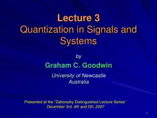
Lecture 3 Quantization in Signals and Systems. by Graham C. Goodwin University of Newcastle Australia. Presented at the “Zaborszky Distinguished Lecture Series” December 3rd, 4th and 5th, 2007. Overview. Topics to be covered include: signal quantization,

E N D
Lecture 3Quantization in Signals and Systems by Graham C. Goodwin University of Newcastle Australia Presented at the “Zaborszky Distinguished Lecture Series” December 3rd, 4th and 5th, 2007
Overview Topics to be covered include: • signal quantization, • predictive and noise shaping quantizers, • networked control, • signal coding in networked control, • channel capacity issues in networked control, • applications in audio compression and control over communication channels.
Outline • Recall Quantization • Predictive and Noise Shaping Quantizers • Application to Audio Compression • Networked Control • Modelling Communication Link • Predictive and Noise Shaping Coding • Experimental Results • Conclusions
Recall Basic Idea of Samplingand Quantization Quantization t t1 t3 0 t2 t4 Sampling
Quantization (Actually we saw some aspects of this in relation to coefficient quantization in lecture 2.) Here: Fix the sampling pattern (say uniform for simplicity) and examine the quantization of the samples. Approaches: • Nonlinear – quantization is an inherently nonlinear process. • Linear – approximate quantization errors as noise. To illustrate ideas we will follow route 2. (Generally gives design insights.)
Signal to Noise Ratio Model for Quantization b = 3 L = 7 b bit quantizer levels Assume quantization errors are white noise uniformly distributed We want small probability that signal amplitude exceeds the range of the quantizer. Assume variance of signal is , then e.g. 4 s.d. rule says that . Hence Q range Uniform Quantizer
Outline • Quantization • Predictive and Noise Shaping Quantizers • Application to Audio Compression • Networked Control • Modelling Communication Link • Predictive and Noise Shaping Coding • Experimental Results • Conclusions
Predictive and Noise Shaping Quantizers (Quantization errors modeled as additive white noise) N C D U E + - L1 L3 Quantizer L2 Utilizing the power of feedback! Note that the feedback loop is related to the delta operator (lecture 2) since we subtract what we already “know” before quantizing/approximating. (We will return to this approximation later!)
Focus on Frequency Weighted (W) Noise Power in D where is the input signal spectrum Use normalized transfer functions; G(0) = 1
Heuristic Explanation of the Optimal Design N • Spectrum of C and characteristics of W are known. • We have 3 filters to design. • One degree of freedom removed by “Perfect Reconstruction” requirement i.e., • With remaining 2 degrees of freedom can (i) shape E to have minimal variance (prediction) and (ii) shape component of due to N to have minimal variance (noise shaping). C D U E + - L1 L3 W Quantizer L2
Perfect Reconstruction Constraint • Minimizing variance of E • Minimize variance of WD due to N • Solution: (Whitening Filter: Predictive coding) (Noise shaping)
Predictive Coder Choose W = 1 Optimal choices are This solution corresponds to Minimum Variance Control
Noise Shaping Quantizer(Sigma-delta) Add extra constraint L3= 1 Optimal Choices: Then(Noise Shaping) (Achieved Performance)
Then apparently, all we need do is make an ideal high pass filter to “push” “quantization noise” outside the band of interest. Does this make sense? The Role of Oversampling Say we choose L3 = 1 and W as ideal low pass filter W 1
Insights from Feedback Theory is a sensitivity function. We know from Bode integral that (Water Bed Effect) Thus making the sensitivity arbitrarily small in some frequency range automatically means that it will be arbitrarily large somewhere else!
Indeed, this goes back to the early simplifying assumption that In fact it should have been and Noise Power in More Complex (but more realistic) optimization problem. It turns out to be convex!
In summary – we can design an “optimal” quantizer which: • minimizes the impact of quantization noise on the output, and • takes account of the fact that quantization errors ultimately need themselves to be quantized due to the feed back structure.
Outline • Quantization • Predictive and Noise Shaping Quantizers • Application to Audio Compression • Networked Control • Modelling Communication Link • Predictive and Noise Shaping Coding • Experimental Results • Conclusions
Application : Audio Compression Original N=0 N=1 N=2 44.1 kHz Bits 3 Stop Elvis Presley
Other Insights From Control Theory (i) Bode integral Spectrum of Errors due to Quantization
Outline • Quantization • Predictive and Noise Shaping Quantizers • Application to Audio Compression • Networked Control • Modelling Communication Link • Predictive and Noise Shaping Coding • Experimental Results • Conclusions
Network Control Systems • In a Networked Control System (NCS) controller and plant are connected via a communication link. • Therefore, signals transmitted: • Have to be quantized • May be delayed • May get lost • The communication link constitutes a performance bottleneck. • When designing NCS’s the characteristics of the network should be accounted for to ensure acceptable performance levels. • When comparing to traditional control loops, in NCS’s there exist additional degrees of freedom to be designed. • It is useful to investigate: • Architectural issues • Signal coding methods
Networked Control Problem (a) (b)
Nominal Control Design • We will consider the situation where an LTI controller has already been designed for a SISO LTI plant model. • We will refer to this design as the nominal design and we will assume that it gives satisfactory performance in a non-networked setting. • We will show how to minimize the impact of the communication link on closed loop performance.
Design Relations Disturbance d The tracking error is given by: where are the loop sensitivity functions. + + + r y Reference + Plant Output - Controller Plant + n Noise
Design Relationships In non-networked situation we have: • To achieve good reference following and disturbance attenuation, C(z) is typically chosen such that the open loop gain, is large at frequencies where and are significant. • To handle measurement noise and plant model inaccuracies, the open loop gain should be reduced at appropriate frequencies.
Outline • Quantization • Predictive and Noise Shaping Quantizers • Application to Audio Compression • Networked Control • Modelling Communication Link • Predictive and Noise Shaping Coding • Experimental Results • Conclusions
The Communication Link • The novel ingredient in an NCS, when compared to a traditional control loop, is the communication link. • It constitutes a significant bottleneck in the achievable performance. • From a design perspective, this opens the possibility of investigating: NCS Architectures Where do I place the processing power? Signal Coding What information do I send?
Channel Model q zero-mean stationary white noise with variance • We will consider an additive Noise model: w v Channel • The channel has a given signal-to-noise ratio, say SNR: • The above characterization encompasses, e.g., • AWGN channels • Bit-rate limited channels (networks), where transmitted signals are passed through an appropriately scaled memoryless quantizer.
Outline • Quantization • Predictive and Noise Shaping Quantizers • Application to Audio Compression • Networked Control • Modelling Communication Link • Predictive and Noise Shaping Coding • Experimental Results • Conclusions
v w x Recall Predictive and Noise shaping quantizer Noise Shaping Quantizer Use this idea in Source Coding • L1 & L2 become part of source coder • L3 becomes part of the source decoder Make transparent to nominal control loop (i.e., Perfect Reconstruction)
Illustration Channel in the Downlink Communication Link q channel y r w v u - - Noise Shaping NCS Architecture Constraint:
Analysis Hence, variance of output error due to quantization errors is (a) However, from SNR model (b) Now (c)
Expression is essentially as for the Predictive and Noise Shaping Quantizer Design save that now the Weighting Function is determined by the Nominal Loop Sensitivity. • Hence can readily determine optimal values of L1, L2 and L3 as before!
Special Case (Predictive Coding)(PCM) Fix L2 = 0 Then
Relationship to Channel Capacity Constraints • The theory shows that for stability when deploying an AWGN channel, one needs: • On the other hand, the channel capacity of an AWGN channel is: • Therefore, if we redesign the controller, the smallest channel capacity consistent with stability is: where {pi} are the unstable poles of the plant.
Optimal Results 1: PCM Coder in Downlink Optimal performance for the down-link architecture • The minimum loss function is given by: • The optimal encoder satisfies: where kD is any positive (fixed) real number.
Optimal Results 2: Up-Link NCS Architecture • For alternative architecture where the communication system is located in the up-link, i.e., between plant output and controller input. d + + + r y + - Controller Plant + n channel Decoder Encoder Communication Link
Optimal Coding • Proceeding as before, we can characterize optimal coders via: where is the power spectral density of the signal • The corresponding optimal loss function is:
Special Case • Internal Model Control Choose C such that • Random Walk disturbances Then i.e., no need for coding in this special case.
Optimal Results 3:Predictive and Noise Shaping Coder in Downlink • The optimal noise shaping parameters are given by where are generalized Blaschke products for and , respectively.
Some Observations • For PCM coding, if disturbances dominate (r = 0), then up-link and down-link architectures give same optimal performance. • For PCM coding, if |GC| = |D| then optimal coder for up-link case is unity (i.e., no need for coding). • If approximately constant as a function of frequency, then (i.e., PCM optimal), otherwise ‘Predictive Noise Shaping Coding’ necessary to achieve optimal performance.
Outline • Quantization • Predictive and Noise Shaping Quantizers • Application to Audio Compression • Networked Control • Modelling Communication Link • Predictive and Noise Shaping Coding • Experimental Results • Conclusions
1. Simulated Example We consider a continuous time plant given by , sampled ever using a zero order hold at its input. The corresponding discrete time transfer function is We will consider two different reference signals, r1 and r2 with PSD’s given by For the control of G(z) we choose the PI controller
The Case of r1 In this case, is approximately constant for all . Then, the PCM based scheme should have a performance which is close to that of the noise shaping based scheme. Tracking error sample variance as a function of the channel bit-rate (r = r1).
The Case of r2 In this case, is far from being constant. Therefore, the noise shaping coder system outperforms PCM.
Finally, you may wonder about the simplification made by approximating the channel quantization errors (a nonlinear phenomenon) by a SNR constrained noise source. The following figure compares the theoretical tracking error (using the ‘noise model’ expressions) with the practical (empirical) errors.