Download
1 / 21
210 likes | 445 Views
v(t) [V]. 20. t [s]. 0. 0. 2. 4. 6. 8. 10. 12. Sound segment. Voltage ramp waveform. Lecture #7 EGR 261 – Signals and Systems. Read : Ch. 1, Sect. 1-4, 6-8 in Linear Signals & Systems, 2 nd Ed. by Lathi. Signals and Systems Signals

E N D
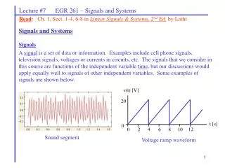
v(t) [V] 20 t [s] 0 0 2 4 6 8 10 12 Sound segment Voltage ramp waveform Lecture #7 EGR 261 – Signals and Systems Read: Ch. 1, Sect. 1-4, 6-8 in Linear Signals & Systems, 2nd Ed. by Lathi Signals and Systems Signals A signal is a set of data or information. Examples include cell phone signals, television signals, voltages or currents in circuits, etc. The signals that we consider in this course are functions of the independent variable time, but our discussions would apply equally well to signals of other independent variables. Some examples of signals are shown below.
System y(t) = Output signal Input signal = x(t) Continuous-time system Lecture #7 EGR 261 – Signals and Systems Systems A system is any process that results in the transformation of signals. A system might have an input signal x(t) and an output signal y(t) as shown below. A system may be made up of physical components, such as in electric circuits or mechanical systems, or a system may be a software algorithm that modifies a signal. Signal Energy and Signal Power Two useful measures of the “size” of a signal are signal energy and signal power.
Lecture #7 EGR 261 – Signals and Systems Signal Energy Signal energy, Ex, is defined as the area under x2(t). For example, signal energy for f(t) shown below is the shaded area shown under f2(t). Ex is defined mathematically as follows:
Lecture #7 EGR 261 – Signals and Systems Signal Power Signal energy must be finite in order for it to be a meaningful measure of signal size. If energy is to be finite, then the signal amplitude must decay, or it is required that signal energy 0 as |t| so that the integral will converge. When signal energy is infinite, a more meaningful measure of the size of a signal is power. Signal power, Px, is the time average of the energy. Px is defined mathematically as follows: For periodic signals with period T, Px is defined as:
Lecture #7 EGR 261 – Signals and Systems RMS value of a signal Since Px is the time average (mean) of the signal amplitude squared, it is also referred to as the mean-squared value of x(t). The square root of this quantity would be the root mean-squared value of x(t) defined as: Units Note that the units for signal energy, Ex, and signal power, Px, are not correct dimensionally. Ex has units of V2s if x(t) is a voltage rather than joules (V2s/) and Ex has units A2s if x(t) is a current rather than joules (A2s). Similarly, Px has units of V2 or I2 rather than watts (V2/ or A2). The units for Ex and Px are dimensionally correct, however, if we think of x(t) as the voltage across a 1 resistor or i(t) as the current through a 1 resistor. So Ex and Px should perhaps be thought of as the energy or power “capability” of the signal, rather than the actual energy or power.
Lecture #7 EGR 261 – Signals and Systems Reference: Linear Signals and Systems, 2nd Edition, by Lathi.
Lecture #7 EGR 261 – Signals and Systems Energy signals and power signals Energy signals have finite energy. All energy signals decay to zero as |t| . Power signals have finite and non-zero power. All periodic signals are power signals. Quiz: Are all energy signals also power signals? No. Any signal with finite energy will have zero power. Are all power signals also energy signals? No. Any signal with non-zero power will have infinite energy. Are all signals either energy signals or power signals? No. Any infinite-duration, increasing-magnitude function will not be either. (For example, the signal x(t) =t is neither.)
A) x(t) 20 10 t -4 0 4 x(t) 20 t 0 4 Lecture #7 EGR 261 – Signals and Systems Example Find the energy or power (whichever is most suitable) for each signal below. B)
C) x(t) x(t) 20 20 t t -4 -4 0 0 4 4 Lecture #7 EGR 261 – Signals and Systems Example (continued) Find the energy or power (whichever is most suitable) for each signal below. D)
x(t) C t q -C Lecture #7 EGR 261 – Signals and Systems Example Find the power and rms value of x(t) = Csin(wt - ) shown below. See the next slide for any trigonometric identities that are required. Result: For any sinusoidal waveform, RMS value = __________________
Lecture #7 EGR 261 – Signals and Systems Trigonometric Identities If any trigonometric identities are required for homework problems, refer to section B.7-6 in Linear Signals and Systems, 2nd Edition, by Lathi. If any of the identities are needed for a test, they will be provided.
Lecture #7 EGR 261 – Signals and Systems • RMS Values of waveforms • We won’t use RMS values much in this course, but they are important in some areas such as in AC circuit analysis. • RMS values of currents and voltages are commonly used in AC circuits. • Most AC meters read RMS values rather than peak values. • Example: A typical household wall outlet has 120V RMS and frequency f = 60 Hz. • Describe this voltage as a sinusoidal function • Sketch the waveform and the RMS value • Find the period, T, and the radian frequency, w. • Show how the RMS value is used to calculate power and compare it to an equivalent DC circuit.
x(t) 10 t 3 1 2 -1 0 x1(t) = x(t - 1) t -1 1 2 0 3 x2(t) = x(t + 1) t 2 -1 1 0 3 Lecture #7 EGR 261 – Signals and Systems • Useful Signal Operations • Three useful signal operations are • discussed below: • Time shifting • Time scaling • Time reversal (inversion) Example: Given x(t) below, sketch x1(t) = x(t – 1) and x2(t) = x(t + 1). Time shifting Consider a signal x(t). x1(t) = x(t – T) is the same signal delayed by T seconds. x2(t) = x(t + T) is the same signal advanced by T seconds. In general, a negative shift is a shift to the right. Similarly, a positive shift is a shift to the left. Replacing every t in a waveform with t – T shifts the waveform T seconds to the right.
Example x(t) Original signal 10 t T2 T1 0 (t) = x(2t) Compressed signal (a = 2) t 0 (t) = x(t/2) Expanded signal (a = 0.5) t 2T1 0 2T2 Lecture #7 EGR 261 – Signals and Systems Time scaling Time scaling is the compression or expansion of a signal. Compressed signal (t) = x(2t) is a compressed version of x(t) as shown on the right. In general, (t) = x(at) represents a compressed signal if a > 1. Expanded signal Similarly, (t) = x(at) represents an expanded signal if a < 1. 10 10 To scale any function by a, replace each t by at in the function.
x(t) 10 t 3 1 2 -1 0 x1(t) = x(2t) t -1 1 2 0 3 x2(t) = x(t/2) t 2 -1 1 0 3 Lecture #7 EGR 261 – Signals and Systems Example: Given x(t) below, sketch x1(t) = x(2t) and x2(t) = x(0.5t) = x(t/2).
x(t) t 1.5 0.5 1.0 -0.5 0 x1(t) = x(2t) t -0.5 0 0.5 1.0 1.5 x2(t) = x(t/2) t 1.0 -0.5 0 0.5 1.5 Lecture #7 EGR 261 – Signals and Systems Example: If x(t) = 10sin(4t - ), sketch x(t), x1(t) = x(2t), and x2(t) = x(t/2). Effect of time scaling on frequency: _________________________________ Effect of time scaling on amplitude: _________________________________ Effect of time scaling on phase: _____________________________________
Example x(t) 10 t 0 x(-t) 10 t 0 Lecture #7 EGR 261 – Signals and Systems Time reversal (inversion) To time-reverse a signal, replace every t with –t. So, x(-t) represents the time reversal (or inverse) of x(t). The graph of x(-t) can be formed by rotating the graph of x(t) 180 about the y-axis.
x(t) 10 t -3 3 -2 1 2 -1 0 x(-t) t -3 3 -2 1 2 -1 0 Lecture #7 EGR 261 – Signals and Systems Example: Given x(t) below, sketch x(-t).
Lecture #7 EGR 261 – Signals and Systems Combined operations We can use various combinations of the three operations just covered: time shifting, time scaling, and time reversal. The operations can often be applied in different orders, but care must be taken. • Example: To form x(at - b) from x(t) we could use two approaches: • Time-shift then time-scale • Time-shift x(t) by b to obtain x(t - b). I.e., replace every t by t - b. • Time-scale x(t - b) by a (i.e., replace t by at) to form x(at - b) • Time-scale then time-shift • Time-scale x(t) by a to obtain x(at). • Time-shift x(at) by b/a (i.e., replace t with t – b/a) to yield • x(a[t – b/a]) = x(at – b)
x(t) 10 t 3 1 2 -1 0 x1(t) = x(2t - 1) t -1 1 2 0 3 x2(t) = x(t/2 + 1) t 2 -1 1 0 3 Lecture #7 EGR 261 – Signals and Systems Example: Given x(t) below, sketch x1(t) = x(2t - 1) and x2(t) = x(t/2 + 1).
Lecture #7 EGR 261 – Signals and Systems Example: Given x(t) and y(t) below, express y(t) in terms of x(t) y(t) x(t) 12 4 0 t 0 t 4 0 2 0


