Signals and Systems
680 likes | 1.65k Views
Signals and Systems. Dr. Mohamed Bingabr University of Central Oklahoma Some of the Slides For Lathi’s Textbook Provided by Dr. Peter Cheung. Course Objectives. • Signal analysis (continuous-time ) • System analysis (mostly continuous systems)

Signals and Systems
E N D
Presentation Transcript
Signals and Systems Dr. Mohamed Bingabr University of Central Oklahoma Some of the Slides For Lathi’s Textbook Provided by Dr. Peter Cheung
Course Objectives • Signal analysis (continuous-time) • System analysis (mostly continuous systems) • Time-domain analysis (including convolution) • Laplace Transform and transfer functions • Fourier Series analysis of periodic signal • Fourier Transform analysis of aperiodic signal • Sampling Theorem and signal reconstructions
Outline • Size of a signal • Useful signal operations • Classification of Signals • Signal Models • Systems • Classification of Systems • System Model: Input-Output Description • Internal and External Description of a System
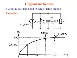
Size of Signal-Energy Signal • Signal: is a set of data or information collected over time. • Measured by signal energy Ex: • Generalize for a complex valued signal to: • Energy must be finite, which means
Size of Signal-Power Signal • If amplitude of x(t) does not 0 when t ", need to measure power Px instead: • Again, generalize for a complex valued signal to:
Useful Signal Operation-Time Delay Find x(t-2) and x(t+2) for the signal x(t) 2 t 1 4
Useful Signal Operation-Time Delay Signal may be delayed by time T: (t) = x (t – T) or advanced by time T: (t) = x (t + T)
Useful Signal Operation-Time Scaling Find x(2t) and x(t/2) for the signal x(t) 2 t 1 4
Useful Signal Operation-Time Scaling Signal may be compressed in time (by a factor of 2): (t) = x (2t) or expanded in time (by a factor of 2): (t) = x (t/2) Same as recording played back at twice and half the speed respectively
Useful Signal Operation-Time Reversal Signal may be reflected about the vertical axis (i.e. time reversed): (t) = x (-t)
Useful Signal Operation-Example We can combine these three operations. For example, the signal x(2t - 6) can be obtained in two ways; • Delay x(t) by 6 to obtain x(t - 6), and then time-compress this signal by factor 2 (replace t with 2t) to obtain x(2t - 6). • Alternately, time-compress x(t) by factor 2 to obtain x(2t), then delay this signal by 3 (replace t with t - 3) to obtain x(2t - 6).
Signal Classification Signals may be classified into: 1. Continuous-time and discrete-time signals 2. Analogue and digital signals 3. Periodic and aperiodic signals 4. Energy and power signals 5. Deterministic and probabilistic signals 6. Causal and non-causal 7. Even and Odd signals
Signal Classification- Continuous vs Discrete Continuous-time Discrete-time
Signal Classification- Analogue vs Digital Analogue, continuous Digital, continuous Analogue, discrete Digital, discrete
Signal Classification- Periodic vsAperiodic A signal x(t) is said to be periodic if for some positive constant To x(t) = x (t+To) for all t The smallest value of To that satisfies the periodicity condition of this equation is the fundamental period of x(t).
Signal Classification- Deterministic vs Random Deterministic Random
Signal Models – Unit Step Function u(t) Step function defined by: Useful to describe a signal that begins at t = 0 (i.e. causal signal). For example, the signal e-at represents an everlasting exponential that starts at t = -. The causal for of this exponential e-atu(t)
Signal Models – Pulse Signal A pulse signal can be presented by two step functions: x(t) = u(t-2) – u(t-4)
Signal Models – Unit Impulse Function δ(t) First defined by Dirac as:
Multiplying Function (t) by an Impulse Since impulse is non-zero only at t = 0, and (t) at t = 0 is (0), we get: We can generalize this for t = T:
Sampling Property of Unit Impulse Function Since we have: It follows that: This is the same as “sampling” (t) at t = 0. If we want to sample (t) at t = T, we just multiple (t) with This is called the “sampling or sifting property” of the impulse.
Examples Simplify the following expression Evaluate the following Find dx/dt for the following signal x(t) = u(t-2) – 3u(t-4)
The Exponential Function est This exponential function is very important in signals & systems, and the parameter s is a complex variable given by:
The Exponential Function est If = 0, then we have the function ejωt, which has a real frequency of ω Therefore the complex variable s = +jωis the complex frequency The function est can be used to describe a very large class of signals and functions. Here are a number of example:
The Complex Frequency Plane s= + jω A real function xe(t) is said to be an even function of t if A real function xo(t) is said to be an odd function of t if HW1_Ch1: 1.1-3, 1.1-4, 1.2-2(a,b,d), 1.2-5, 1.4-3, 1.4-4, 1.4-5, 1.4-10 (b, f)
Even and Odd Function Even and odd functions have the following properties: • Even x Odd = Odd • Odd x Odd = Even • Even x Even = Even Every signal x(t) can be expressed as a sum of even and odd components because:
Even and Odd Function Consider the causal exponential function
What are Systems? • Systems are used to process signals to modify or extract information • Physical system – characterized by their input-output relationships • E.g. electrical systems are characterized by voltage-current relationships • From this, we derive a mathematical model of the system • “Black box” model of a system:
Classification of Systems Systems may be classified into: Linear and non-linear systems Constant parameter and time-varying-parameter systems Instantaneous (memoryless) and dynamic (with memory) systems Causal and non-causal systems Continuous-time and discrete-time systems Analogue and digital systems Invertible and noninvertible systems Stable and unstable systems
Linear Systems (1) • A linear system exhibits the additivity property: • if and then • It also must satisfy the homogeneity or scaling property: • if then • These can be combined into the property of superposition: • if and then • A non-linear system is one that is NOT linear (i.e. does not obey the principle of superposition)
Linear Systems (4) Is the system y = x2 linear?
Linear Systems (5) A complex input can be represented as a sum of simpler inputs (pulse, step, sinusoidal), and then use linearity to find the response to this simple inputs to find the system output to the complex input.
Time-Invariant System Which of the system is time-invariant? (a) y(t) = 3x(t) (b) y(t) = t x(t)
Causal and Noncausal Systems Which of the two systems is causal? a) y(t) = 3 x(t) + x(t-2) b) y(t) = 3x(t) + x(t+2)
Invertible and Noninvertible Which of the two systems is invertible? y(t) = x2 y= 2x
Electrical System + v(t) - i(t) R + v(t) - i(t) i(t) + v(t) -
Linear Differential Systems (2) Find the input-output relationship for the transational mechanical system shown below. The input is the force x(t), and the output is the mass position y(t)
Linear Differential Systems (4) HW2_Ch1: 1.7-1 (a, b, d), 1.7-2 (a, b, c), 1.7-7, 1.7-13, 1.8-1, 1.8-3