Download
1 / 32
320 likes | 484 Views
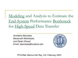
Modeling and Analysis to Estimate the End-System Performance Bottleneck for High-Speed Data Transfer. Amitabha Banerjee, Biswanath Mukherjee, and Dipak Ghosal Email: abanerjee@ucdavis.edu. PFLDNet , Marina Del Rey, CA, February 2007. Outline. Motivation End-System Model

E N D
Modeling and Analysis to Estimate the End-System Performance Bottleneck for High-Speed Data Transfer Amitabha Banerjee, Biswanath Mukherjee, and Dipak Ghosal Email: abanerjee@ucdavis.edu PFLDNet, Marina Del Rey, CA, February 2007.
Outline • Motivation • End-System Model • Analytical & Experimental Results • Conclusions & Future Work
Key Development in Network Technologies • Backbone: • Lambda-Grids: Up to 10 Gbps (OC-192) circuits. e.g., National Lambda Rail, DoE UltraScienceNet • Access: • Passive Optical Networks: 1/10 Gig EPON. • Adapters: • 1/10 Gig Network Adapters. • Standardization of 100 Gig Ethernet. • With these we have the ability to establish: • High-capacity end-to-end connections. • End-to-end dedicated circuits.
Limited End-System Capacity • Disk Speeds: • SATA: 2.4 Gbps (3.0 Gbps reduced by 8/10 coding.) • Bus Speeds: • 133 MHz 64-bit PCI-X: 8.5 Gbps • PCI-E is much faster (8 GBps) • Memory/ Cache contentions. • Overloaded CPU (Particularly in single processor environments) End-system not keeping pace with the network
End-System Bottleneck Operations on Received Packet • DMA’ed to Memory. • Processed in Network Protocol Stack. • Copied from Kernel-space to User-space, Delivered to Socket Buffer. • Read by Application, Processed, Written to Disk, etc. High-speed Network
Experiments with UDT Idle System Pentium IV 3 GHz, 2 GB RAM 1 Gig E network, RAMDisk-RAMDisk Transfer One loop Two loops
Review of Flow Control Mechanisms • TCP • Receiver Advertises Empty Socket Buffer (Flow Window). • Sender limits Un-Acked packets to Flow Window size. • LambdaStream • Measures packet inter-arrival time. Compares with sending inter-arrival time. • Sends feedback whether to increase/ reduce sending rate.
Limitations of Existing Flow Control Mechanisms • Operates only at Socket – Application Interface. • OS and NIC semantics not captured. • Bursty and transient metrics. • Application reads data in bursts. • When RTT is high, information is stale for sender, particularly when it is very transient.
Our Goal • Achieve End-System Performance Aware Flow Control • Model all possible bottlenecks at end-system. • Estimate best data transfer rate considering entire end-system performance. • This rate, the effective bottleneck rate, is derived as function of current workload. • Match sending rate to effective bottleneck rate. • Merits: • Workload: Less transient => More reliable data. • Rate Matching across all end-system components.
Outline • Motivation • End-System Model • Analytical & Experimental Results • Conclusions & Future Work
Markov Models • Markov Models: Stochastic Analysis of System Performance • Tools to create Markov Models: • Petri Nets, introduced in 1962. • Stochastic Petri Nets (SPN), • Stochastic Reward Nets (SRN) • Allows for Automatic Generation of Markov chains from any of the above models. • Tools: SPNP, SHARPE, MOSEL 2, etc.
Categorize Tasks • CPU-bound tasks • Uses CPU cycles constantly. • I/O-bound tasks • Uses CPU and I/O alternately. • Network tasks • Requires processing of ISRs.
#i SRN Model of End-System (Memory-to-Memory Data Transfer) tdisk tcpu I - #i Representation of I/O bound task pdisk pcpu PS FCFS tcpu: Transition for CPU processing #C: Number of CPU-bound tasks tdisk: Transition for Disk processing #I: Number of I/O-bound tasks Steady State Analysis => Probability of I/O Task Distribution Workload
#i tcpu A Representation of Network I/O Interrupt Process As a Tagged Customer S Absorption State Guard: All transitions stop when task reaches Absorption State PS SRN Model of End-System (Memory-to-Memory Data Transfer) tdisk tcpu Representation of I/O bound task pdisk pcpu PS FCFS tcpu: Transition for CPU processing tdisk: Transition for Disk processing #C=Number of CPU-bound tasks
Transient Analysis of SRN Model • Yields Response-Time Distribution from states ‘S’ to ‘A’ as function of Workload • Derive Expected Rate of ISR service Workload
SPN Model of NIC K (N) Corresponds to bulk-service due to interrupt coalescing Corresponds to servicing the ISR (Computed from response-time Distribution of a Tagged Customer) N K Corresponds to finite buffer SPN model is employed to determine packet loss as function of
Estimation of Effective Bottleneck Rate Time required to transmit first burst Time to send subsequent bursts Time to send error sequence numbers l T B*send Bsend B*send Bsend
How to Determine Model Parameters • Representative Workloads • I/O-bound Task: Task reading random line from file. • Network I/O Task: Task reading data from network. • Use MAGNET to trace above task • Determine service time distributions at CPU & disk • Determine Expected Service Rates from these distributions • Approximations • Capture high-level stochastic metrics. • Leave out OS & Task specific implementation details. • Simple model which can be easily developed and analyzed in software.
Outline • Motivation • End-System Model • Analytical & Experimental Results • Conclusions & Future Work
Discussion • Proposed an approach to achieve End-System Performance Aware Flow Control • Illustrated model for memory-to-memory data transfer. Similar models possible for other scenarios. • Demonstrated that Analytical model yields effective bottleneck rate as function of workload.
Challenges • How to implement in software? • Analytical model parameters to be determined only ONCE. Therefore, measure statically (At time of software installation). • Construct SRN model at runtime. • Workload determined at time of data transfer. • Determine tasks, classify them CPU-bound & I/O-bound. • Monitor changes in workload. • Deliver feedback on effective bottleneck rate. (TCP) • Match sending rate to receiver bottleneck. (Pacing)
Receiving data • Data Analysis/ • Visualization • Other I/O • Interrupt Handling S Lambda-Grid R S S Potential End-System Congestion High-Speed Networks => No Network Congestion End-To-End Data Transfer
Application-to-Application data transfer p1 t1 #i Representation of application process Processor: PS t2 pa1 pa2 S A Representation of network I/O process Processor: PS Processor: PS
Disk-to-Disk data transfer pd1 t1 #i Representation of I/O process Processor: PS Disk: FCFS pd2 t2 S A Representation of network I/O process Processor: PS Disk: FCFS